Import and Tidy Data

Biostat 203B

Display machine information for reproducibility.

R

sessionInfo()

R version 4.2.2 (2022-10-31)
Platform: x86_64-apple-darwin17.0 (64-bit)
Running under: macOS Big Sur ... 10.16

Matrix products: default
BLAS:   /Library/Frameworks/R.framework/Versions/4.2/Resources/lib/libRblas.0.dylib
LAPACK: /Library/Frameworks/R.framework/Versions/4.2/Resources/lib/libRlapack.dylib

locale:
[1] en_US.UTF-8/en_US.UTF-8/en_US.UTF-8/C/en_US.UTF-8/en_US.UTF-8

attached base packages:
[1] stats     graphics  grDevices utils     datasets  methods   base     

loaded via a namespace (and not attached):
 [1] digest_0.6.30     lifecycle_1.0.3   jsonlite_1.8.4    magrittr_2.0.3   
 [5] evaluate_0.18     rlang_1.0.6       stringi_1.7.8     cli_3.4.1        
 [9] rstudioapi_0.14   vctrs_0.5.1       rmarkdown_2.18    tools_4.2.2      
[13] stringr_1.5.0     glue_1.6.2        htmlwidgets_1.6.0 xfun_0.35        
[17] yaml_2.3.6        fastmap_1.1.0     compiler_4.2.2    htmltools_0.5.4  
[21] knitr_1.41       

Python

import IPython
print(IPython.sys_info())

{'commit_hash': 'add5877a4',
 'commit_source': 'installation',
 'default_encoding': 'utf-8',
 'ipython_path': '/Library/Frameworks/Python.framework/Versions/3.10/lib/python3.10/site-packages/IPython',
 'ipython_version': '8.8.0',
 'os_name': 'posix',
 'platform': 'macOS-10.16-x86_64-i386-64bit',
 'sys_executable': '/Library/Frameworks/Python.framework/Versions/3.10/bin/python3',
 'sys_platform': 'darwin',
 'sys_version': '3.10.9 (v3.10.9:1dd9be6584, Dec  6 2022, 14:37:36) [Clang '
                '13.0.0 (clang-1300.0.29.30)]'}

Julia

using InteractiveUtils
versioninfo()

Julia Version 1.8.3
Commit 0434deb161e (2022-11-14 20:14 UTC)
Platform Info:
  OS: macOS (x86_64-apple-darwin21.4.0)
  CPU: 8 × Intel(R) Core(TM) i7-6920HQ CPU @ 2.90GHz
  WORD_SIZE: 64
  LIBM: libopenlibm
  LLVM: libLLVM-13.0.1 (ORCJIT, skylake)
  Threads: 1 on 8 virtual cores
Environment:
  DYLD_FALLBACK_LIBRARY_PATH = /Library/Frameworks/R.framework/Resources/lib:/Library/Java/JavaVirtualMachines/jdk1.8.0_241.jdk/Contents/Home/jre/lib/server
  JULIA_EDITOR = code

1 Outline

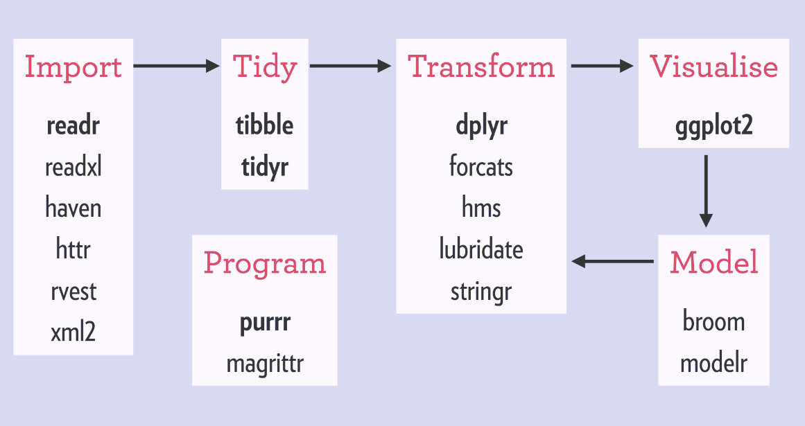
We will spend the next few weeks studying some R packages for typical data science projects.

• Data wrangling (import, tidy, visualization, transformation).

  • R for Data Science by Garrett Grolemund and Hadley Wickham.
  • R Graphics Cookbook by Winston Chang.

• Interactive data visualization by Shiny.

• Interface with databases, e.g., SQL, Google BigQuery, and Apache Spark.

• String and text data manipulation.

• Web scraping.

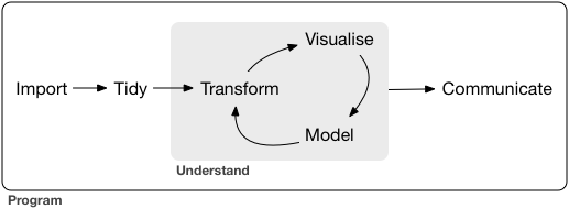
A typical data science project:

2 Tidyverse

R

• tidyverse is a collection of R packages for data ingestion, wrangling, and visualization.

• The lead developer Hadley Wickham won the 2019 COPSS Presidents’ Award (the Nobel Prize of Statistics)

for influential work in statistical computing, visualization, graphics, and data analysis; for developing and implementing an impressively comprehensive computational infrastructure for data analysis through R software; for making statistical thinking and computing accessible to large audience; and for enhancing an appreciation for the important role of statistics among data scientists.

• Install tidyverse from RStudio menu Tools -> Install Packages... or

install.packages("tidyverse")

• After installation, load tidyverse by

library("tidyverse")

── Attaching packages ─────────────────────────────────────── tidyverse 1.3.2 ──
✔ ggplot2 3.4.0      ✔ purrr   1.0.0 
✔ tibble  3.1.8      ✔ dplyr   1.0.10
✔ tidyr   1.2.1      ✔ stringr 1.5.0 
✔ readr   2.1.3      ✔ forcats 0.5.2 
── Conflicts ────────────────────────────────────────── tidyverse_conflicts() ──
✖ dplyr::filter() masks stats::filter()
✖ dplyr::lag()    masks stats::lag()

Python

The pandas package is the Python analog of tidyverse.

Follow the installation instructions to install pandas package in Python.

Julia

The DataFrames.jl package and the JuliaData ecosystem is the Julia analog of tidyverse.

Install DataFrames.jl by:

add DataFrames

in the package mode or

using Pkg
Pkg.add("DatamFrames")

in Julia REPL.

3 Tibble | r4ds chapter 10

3.1 Tibbles

• Tibbles extend data frames in R and form the core of tidyverse.

3.2 Create tibbles

3.2.1 Convert between dataframe in base R and tibble

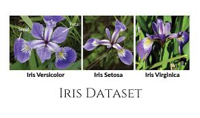
• iris is a data frame available in base R:

# By default, R displays ALL rows of a regular data frame!
iris

    Sepal.Length Sepal.Width Petal.Length Petal.Width    Species
1            5.1         3.5          1.4         0.2     setosa
2            4.9         3.0          1.4         0.2     setosa
3            4.7         3.2          1.3         0.2     setosa
4            4.6         3.1          1.5         0.2     setosa
5            5.0         3.6          1.4         0.2     setosa
6            5.4         3.9          1.7         0.4     setosa
7            4.6         3.4          1.4         0.3     setosa
8            5.0         3.4          1.5         0.2     setosa
9            4.4         2.9          1.4         0.2     setosa
10           4.9         3.1          1.5         0.1     setosa
11           5.4         3.7          1.5         0.2     setosa
12           4.8         3.4          1.6         0.2     setosa
13           4.8         3.0          1.4         0.1     setosa
14           4.3         3.0          1.1         0.1     setosa
15           5.8         4.0          1.2         0.2     setosa
16           5.7         4.4          1.5         0.4     setosa
17           5.4         3.9          1.3         0.4     setosa
18           5.1         3.5          1.4         0.3     setosa
19           5.7         3.8          1.7         0.3     setosa
20           5.1         3.8          1.5         0.3     setosa
21           5.4         3.4          1.7         0.2     setosa
22           5.1         3.7          1.5         0.4     setosa
23           4.6         3.6          1.0         0.2     setosa
24           5.1         3.3          1.7         0.5     setosa
25           4.8         3.4          1.9         0.2     setosa
26           5.0         3.0          1.6         0.2     setosa
27           5.0         3.4          1.6         0.4     setosa
28           5.2         3.5          1.5         0.2     setosa
29           5.2         3.4          1.4         0.2     setosa
30           4.7         3.2          1.6         0.2     setosa
31           4.8         3.1          1.6         0.2     setosa
32           5.4         3.4          1.5         0.4     setosa
33           5.2         4.1          1.5         0.1     setosa
34           5.5         4.2          1.4         0.2     setosa
35           4.9         3.1          1.5         0.2     setosa
36           5.0         3.2          1.2         0.2     setosa
37           5.5         3.5          1.3         0.2     setosa
38           4.9         3.6          1.4         0.1     setosa
39           4.4         3.0          1.3         0.2     setosa
40           5.1         3.4          1.5         0.2     setosa
41           5.0         3.5          1.3         0.3     setosa
42           4.5         2.3          1.3         0.3     setosa
43           4.4         3.2          1.3         0.2     setosa
44           5.0         3.5          1.6         0.6     setosa
45           5.1         3.8          1.9         0.4     setosa
46           4.8         3.0          1.4         0.3     setosa
47           5.1         3.8          1.6         0.2     setosa
48           4.6         3.2          1.4         0.2     setosa
49           5.3         3.7          1.5         0.2     setosa
50           5.0         3.3          1.4         0.2     setosa
51           7.0         3.2          4.7         1.4 versicolor
52           6.4         3.2          4.5         1.5 versicolor
53           6.9         3.1          4.9         1.5 versicolor
54           5.5         2.3          4.0         1.3 versicolor
55           6.5         2.8          4.6         1.5 versicolor
56           5.7         2.8          4.5         1.3 versicolor
57           6.3         3.3          4.7         1.6 versicolor
58           4.9         2.4          3.3         1.0 versicolor
59           6.6         2.9          4.6         1.3 versicolor
60           5.2         2.7          3.9         1.4 versicolor
61           5.0         2.0          3.5         1.0 versicolor
62           5.9         3.0          4.2         1.5 versicolor
63           6.0         2.2          4.0         1.0 versicolor
64           6.1         2.9          4.7         1.4 versicolor
65           5.6         2.9          3.6         1.3 versicolor
66           6.7         3.1          4.4         1.4 versicolor
67           5.6         3.0          4.5         1.5 versicolor
68           5.8         2.7          4.1         1.0 versicolor
69           6.2         2.2          4.5         1.5 versicolor
70           5.6         2.5          3.9         1.1 versicolor
71           5.9         3.2          4.8         1.8 versicolor
72           6.1         2.8          4.0         1.3 versicolor
73           6.3         2.5          4.9         1.5 versicolor
74           6.1         2.8          4.7         1.2 versicolor
75           6.4         2.9          4.3         1.3 versicolor
76           6.6         3.0          4.4         1.4 versicolor
77           6.8         2.8          4.8         1.4 versicolor
78           6.7         3.0          5.0         1.7 versicolor
79           6.0         2.9          4.5         1.5 versicolor
80           5.7         2.6          3.5         1.0 versicolor
81           5.5         2.4          3.8         1.1 versicolor
82           5.5         2.4          3.7         1.0 versicolor
83           5.8         2.7          3.9         1.2 versicolor
84           6.0         2.7          5.1         1.6 versicolor
85           5.4         3.0          4.5         1.5 versicolor
86           6.0         3.4          4.5         1.6 versicolor
87           6.7         3.1          4.7         1.5 versicolor
88           6.3         2.3          4.4         1.3 versicolor
89           5.6         3.0          4.1         1.3 versicolor
90           5.5         2.5          4.0         1.3 versicolor
91           5.5         2.6          4.4         1.2 versicolor
92           6.1         3.0          4.6         1.4 versicolor
93           5.8         2.6          4.0         1.2 versicolor
94           5.0         2.3          3.3         1.0 versicolor
95           5.6         2.7          4.2         1.3 versicolor
96           5.7         3.0          4.2         1.2 versicolor
97           5.7         2.9          4.2         1.3 versicolor
98           6.2         2.9          4.3         1.3 versicolor
99           5.1         2.5          3.0         1.1 versicolor
100          5.7         2.8          4.1         1.3 versicolor
101          6.3         3.3          6.0         2.5  virginica
102          5.8         2.7          5.1         1.9  virginica
103          7.1         3.0          5.9         2.1  virginica
104          6.3         2.9          5.6         1.8  virginica
105          6.5         3.0          5.8         2.2  virginica
106          7.6         3.0          6.6         2.1  virginica
107          4.9         2.5          4.5         1.7  virginica
108          7.3         2.9          6.3         1.8  virginica
109          6.7         2.5          5.8         1.8  virginica
110          7.2         3.6          6.1         2.5  virginica
111          6.5         3.2          5.1         2.0  virginica
112          6.4         2.7          5.3         1.9  virginica
113          6.8         3.0          5.5         2.1  virginica
114          5.7         2.5          5.0         2.0  virginica
115          5.8         2.8          5.1         2.4  virginica
116          6.4         3.2          5.3         2.3  virginica
117          6.5         3.0          5.5         1.8  virginica
118          7.7         3.8          6.7         2.2  virginica
119          7.7         2.6          6.9         2.3  virginica
120          6.0         2.2          5.0         1.5  virginica
121          6.9         3.2          5.7         2.3  virginica
122          5.6         2.8          4.9         2.0  virginica
123          7.7         2.8          6.7         2.0  virginica
124          6.3         2.7          4.9         1.8  virginica
125          6.7         3.3          5.7         2.1  virginica
126          7.2         3.2          6.0         1.8  virginica
127          6.2         2.8          4.8         1.8  virginica
128          6.1         3.0          4.9         1.8  virginica
129          6.4         2.8          5.6         2.1  virginica
130          7.2         3.0          5.8         1.6  virginica
131          7.4         2.8          6.1         1.9  virginica
132          7.9         3.8          6.4         2.0  virginica
133          6.4         2.8          5.6         2.2  virginica
134          6.3         2.8          5.1         1.5  virginica
135          6.1         2.6          5.6         1.4  virginica
136          7.7         3.0          6.1         2.3  virginica
137          6.3         3.4          5.6         2.4  virginica
138          6.4         3.1          5.5         1.8  virginica
139          6.0         3.0          4.8         1.8  virginica
140          6.9         3.1          5.4         2.1  virginica
141          6.7         3.1          5.6         2.4  virginica
142          6.9         3.1          5.1         2.3  virginica
143          5.8         2.7          5.1         1.9  virginica
144          6.8         3.2          5.9         2.3  virginica
145          6.7         3.3          5.7         2.5  virginica
146          6.7         3.0          5.2         2.3  virginica
147          6.3         2.5          5.0         1.9  virginica
148          6.5         3.0          5.2         2.0  virginica
149          6.2         3.4          5.4         2.3  virginica
150          5.9         3.0          5.1         1.8  virginica

• Convert a regular data frame to tibble, which by default only displays the first 10 rows of data.

as_tibble(iris)

# A tibble: 150 × 5
   Sepal.Length Sepal.Width Petal.Length Petal.Width Species
          <dbl>       <dbl>        <dbl>       <dbl> <fct>  
 1          5.1         3.5          1.4         0.2 setosa 
 2          4.9         3            1.4         0.2 setosa 
 3          4.7         3.2          1.3         0.2 setosa 
 4          4.6         3.1          1.5         0.2 setosa 
 5          5           3.6          1.4         0.2 setosa 
 6          5.4         3.9          1.7         0.4 setosa 
 7          4.6         3.4          1.4         0.3 setosa 
 8          5           3.4          1.5         0.2 setosa 
 9          4.4         2.9          1.4         0.2 setosa 
10          4.9         3.1          1.5         0.1 setosa 
# … with 140 more rows

• Convert a tibble to data frame:

as.data.frame(tb)

3.2.2 Construct tibbles by columns

• Create tibble/dataframe from individual vectors.

R

Note values for y are recycled:

tibble(
  x = 1:5, 
  y = 1, 
  z = x ^ 2 + y
)

# A tibble: 5 × 3
      x     y     z
  <int> <dbl> <dbl>
1     1     1     2
2     2     1     5
3     3     1    10
4     4     1    17
5     5     1    26

Python

# Load the pandas library
import pandas as pd
# Load numpy for array manipulation
import numpy as np

# Create DataFrame from a dictionary
df = pd.DataFrame({
  'x': np.linspace(1, 5, 5), 
  'y': np.ones(5)
  })
df['z'] = df['x']**2 + df['y']
df

     x    y     z
0  1.0  1.0   2.0
1  2.0  1.0   5.0
2  3.0  1.0  10.0
3  4.0  1.0  17.0
4  5.0  1.0  26.0

Julia

using DataFrames

df = DataFrame(
  x = 1:5,
  y = 1,
);
df[!, :z] = df[!, :x].^2 + df[!, :y];
df

5×3 DataFrame
 Row │ x      y      z
     │ Int64  Int64  Int64
─────┼─────────────────────
   1 │     1      1      2
   2 │     2      1      5
   3 │     3      1     10
   4 │     4      1     17
   5 │     5      1     26

3.2.3 Construct tibbles by rows

• Transposed tibbles, or construct dataframe by rows:

R

tribble(
  ~x, ~y, ~z,
  #--|--|----
  "a", 2, 3.6,
  "b", 1, 8.5
)

# A tibble: 2 × 3
  x         y     z
  <chr> <dbl> <dbl>
1 a         2   3.6
2 b         1   8.5

Python

# Initialize list of lists
data = [['a', 2, 3.6], ['b', 1, 8.5]]
# Create DataFrame
df = pd.DataFrame(data, columns = ['x', 'y', 'z'])
df

   x  y    z
0  a  2  3.6
1  b  1  8.5

Julia

In Julia, we can build a DataFrame row by row by pushing tuples

df = DataFrame(x = String[], y = Int[], z = Float64[]);
push!(df, ("a", 2, 3.6));
push!(df, ("b", 1, 8.5));
df

2×3 DataFrame
 Row │ x       y      z
     │ String  Int64  Float64
─────┼────────────────────────
   1 │ a           2      3.6
   2 │ b           1      8.5

or dictionary

df = DataFrame(x = String[], y = Int[], z = Float64[]);
push!(df, Dict(:x => "a", :y => 2, :z => 3.6));
push!(df, Dict(:x => "b", :y => 1, :z => 8.5));
df

2×3 DataFrame
 Row │ x       y      z
     │ String  Int64  Float64
─────┼────────────────────────
   1 │ a           2      3.6
   2 │ b           1      8.5

If you want to add rows at the beginning of a data frame use pushfirst! and to insert a row in an arbitrary location use insert!.

You can also add whole tables to a data frame using the append! and prepend! functions.

3.3 Printing of a tibble

R

• By default, tibble prints the first 10 rows and all columns that fit on screen.

nycflights13::flights

# A tibble: 336,776 × 19
    year month   day dep_time sched_de…¹ dep_d…² arr_t…³ sched…⁴ arr_d…⁵ carrier
   <int> <int> <int>    <int>      <int>   <dbl>   <int>   <int>   <dbl> <chr>  
 1  2013     1     1      517        515       2     830     819      11 UA     
 2  2013     1     1      533        529       4     850     830      20 UA     
 3  2013     1     1      542        540       2     923     850      33 AA     
 4  2013     1     1      544        545      -1    1004    1022     -18 B6     
 5  2013     1     1      554        600      -6     812     837     -25 DL     
 6  2013     1     1      554        558      -4     740     728      12 UA     
 7  2013     1     1      555        600      -5     913     854      19 B6     
 8  2013     1     1      557        600      -3     709     723     -14 EV     
 9  2013     1     1      557        600      -3     838     846      -8 B6     
10  2013     1     1      558        600      -2     753     745       8 AA     
# … with 336,766 more rows, 9 more variables: flight <int>, tailnum <chr>,
#   origin <chr>, dest <chr>, air_time <dbl>, distance <dbl>, hour <dbl>,
#   minute <dbl>, time_hour <dttm>, and abbreviated variable names
#   ¹​sched_dep_time, ²​dep_delay, ³​arr_time, ⁴​sched_arr_time, ⁵​arr_delay

• To change number of rows and columns to display:

nycflights13::flights %>% 
  print(n = 10, width = Inf)

# A tibble: 336,776 × 19
    year month   day dep_time sched_dep_time dep_delay arr_time sched_arr_time
   <int> <int> <int>    <int>          <int>     <dbl>    <int>          <int>
 1  2013     1     1      517            515         2      830            819
 2  2013     1     1      533            529         4      850            830
 3  2013     1     1      542            540         2      923            850
 4  2013     1     1      544            545        -1     1004           1022
 5  2013     1     1      554            600        -6      812            837
 6  2013     1     1      554            558        -4      740            728
 7  2013     1     1      555            600        -5      913            854
 8  2013     1     1      557            600        -3      709            723
 9  2013     1     1      557            600        -3      838            846
10  2013     1     1      558            600        -2      753            745
   arr_delay carrier flight tailnum origin dest  air_time distance  hour minute
       <dbl> <chr>    <int> <chr>   <chr>  <chr>    <dbl>    <dbl> <dbl>  <dbl>
 1        11 UA        1545 N14228  EWR    IAH        227     1400     5     15
 2        20 UA        1714 N24211  LGA    IAH        227     1416     5     29
 3        33 AA        1141 N619AA  JFK    MIA        160     1089     5     40
 4       -18 B6         725 N804JB  JFK    BQN        183     1576     5     45
 5       -25 DL         461 N668DN  LGA    ATL        116      762     6      0
 6        12 UA        1696 N39463  EWR    ORD        150      719     5     58
 7        19 B6         507 N516JB  EWR    FLL        158     1065     6      0
 8       -14 EV        5708 N829AS  LGA    IAD         53      229     6      0
 9        -8 B6          79 N593JB  JFK    MCO        140      944     6      0
10         8 AA         301 N3ALAA  LGA    ORD        138      733     6      0
   time_hour          
   <dttm>             
 1 2013-01-01 05:00:00
 2 2013-01-01 05:00:00
 3 2013-01-01 05:00:00
 4 2013-01-01 05:00:00
 5 2013-01-01 06:00:00
 6 2013-01-01 05:00:00
 7 2013-01-01 06:00:00
 8 2013-01-01 06:00:00
 9 2013-01-01 06:00:00
10 2013-01-01 06:00:00
# … with 336,766 more rows

Here we see the pipe operator %>% pipes the output from previous command to the (first) argument of the next command.

• To change the default print setting globally:
  • options(tibble.print_max = n, tibble.print_min = m): if more than m rows, print only n rows.
  • options(dplyr.print_min = Inf): print all row.
  • options(tibble.width = Inf): print all columns.

Python

Pandas by default displays 10 rows and limits the number of columns to the display area.

from nycflights13 import flights
flights

        year  month  day  ...  hour  minute             time_hour
0       2013      1    1  ...     5      15  2013-01-01T10:00:00Z
1       2013      1    1  ...     5      29  2013-01-01T10:00:00Z
2       2013      1    1  ...     5      40  2013-01-01T10:00:00Z
3       2013      1    1  ...     5      45  2013-01-01T10:00:00Z
4       2013      1    1  ...     6       0  2013-01-01T11:00:00Z
...      ...    ...  ...  ...   ...     ...                   ...
336771  2013      9   30  ...    14      55  2013-09-30T18:00:00Z
336772  2013      9   30  ...    22       0  2013-10-01T02:00:00Z
336773  2013      9   30  ...    12      10  2013-09-30T16:00:00Z
336774  2013      9   30  ...    11      59  2013-09-30T15:00:00Z
336775  2013      9   30  ...     8      40  2013-09-30T12:00:00Z

[336776 rows x 19 columns]

We can override this behavior by

pd.set_option("display.max_rows", 50)
pd.set_option("display.max_columns", 20)

flights

        year  month  day  dep_time  sched_dep_time  dep_delay  arr_time  \
0       2013      1    1     517.0             515        2.0     830.0   
1       2013      1    1     533.0             529        4.0     850.0   
2       2013      1    1     542.0             540        2.0     923.0   
3       2013      1    1     544.0             545       -1.0    1004.0   
4       2013      1    1     554.0             600       -6.0     812.0   
...      ...    ...  ...       ...             ...        ...       ...   
336771  2013      9   30       NaN            1455        NaN       NaN   
336772  2013      9   30       NaN            2200        NaN       NaN   
336773  2013      9   30       NaN            1210        NaN       NaN   
336774  2013      9   30       NaN            1159        NaN       NaN   
336775  2013      9   30       NaN             840        NaN       NaN   

        sched_arr_time  arr_delay carrier  flight tailnum origin dest  \
0                  819       11.0      UA    1545  N14228    EWR  IAH   
1                  830       20.0      UA    1714  N24211    LGA  IAH   
2                  850       33.0      AA    1141  N619AA    JFK  MIA   
3                 1022      -18.0      B6     725  N804JB    JFK  BQN   
4                  837      -25.0      DL     461  N668DN    LGA  ATL   
...                ...        ...     ...     ...     ...    ...  ...   
336771            1634        NaN      9E    3393     NaN    JFK  DCA   
336772            2312        NaN      9E    3525     NaN    LGA  SYR   
336773            1330        NaN      MQ    3461  N535MQ    LGA  BNA   
336774            1344        NaN      MQ    3572  N511MQ    LGA  CLE   
336775            1020        NaN      MQ    3531  N839MQ    LGA  RDU   

        air_time  distance  hour  minute             time_hour  
0          227.0      1400     5      15  2013-01-01T10:00:00Z  
1          227.0      1416     5      29  2013-01-01T10:00:00Z  
2          160.0      1089     5      40  2013-01-01T10:00:00Z  
3          183.0      1576     5      45  2013-01-01T10:00:00Z  
4          116.0       762     6       0  2013-01-01T11:00:00Z  
...          ...       ...   ...     ...                   ...  
336771       NaN       213    14      55  2013-09-30T18:00:00Z  
336772       NaN       198    22       0  2013-10-01T02:00:00Z  
336773       NaN       764    12      10  2013-09-30T16:00:00Z  
336774       NaN       419    11      59  2013-09-30T15:00:00Z  
336775       NaN       431     8      40  2013-09-30T12:00:00Z  

[336776 rows x 19 columns]

Julia

By default DataFrames.jl limits the number of rows and columns when displaying a data frame in a Jupyter Notebook to 25 and 100, respectively. You can override this behavior by changing the values of the ENV["DATAFRAMES_COLUMNS"] and ENV["DATAFRAMES_ROWS"] variables to hold the maximum number of columns and rows of the output. All columns or rows will be printed if those numbers are equal or lower than 0.

3.4 Subsetting

3.4.1 Extract columns

R

• Create a tibble with two columns.

df <- tibble(
  x = runif(5),
  y = rnorm(5)
)
df

# A tibble: 5 × 2
      x      y
  <dbl>  <dbl>
1 0.269  0.467
2 0.983 -0.690
3 0.149 -1.05 
4 0.263  0.211
5 0.894 -1.25 

• Extract a column by name:

# Return a vector
df$x

[1] 0.2688478 0.9827850 0.1490404 0.2630770 0.8938164

# Return a vector
df[["x"]]

[1] 0.2688478 0.9827850 0.1490404 0.2630770 0.8938164

# Return a tibble
df[, "x"]

# A tibble: 5 × 1
      x
  <dbl>
1 0.269
2 0.983
3 0.149
4 0.263
5 0.894

• Extract a column by position. Remember R indexing starts from 1!

# Return a tibble
df[, 1] 

# A tibble: 5 × 1
      x
  <dbl>
1 0.269
2 0.983
3 0.149
4 0.263
5 0.894

# Return a vector
df[[1]] 

[1] 0.2688478 0.9827850 0.1490404 0.2630770 0.8938164

• Pipe:

# Return a vector
df %>% .$x

[1] 0.2688478 0.9827850 0.1490404 0.2630770 0.8938164

# Return a vector
df %>% .[["x"]]

[1] 0.2688478 0.9827850 0.1490404 0.2630770 0.8938164

• Access multiple columns at once.

# Return a tibble
df[, c("x", "y")]

# A tibble: 5 × 2
      x      y
  <dbl>  <dbl>
1 0.269  0.467
2 0.983 -0.690
3 0.149 -1.05 
4 0.263  0.211
5 0.894 -1.25 

# Return a tibble
df[c("x", "y")]

# A tibble: 5 × 2
      x      y
  <dbl>  <dbl>
1 0.269  0.467
2 0.983 -0.690
3 0.149 -1.05 
4 0.263  0.211
5 0.894 -1.25 

# Return a tibble
df[c(1, 2)]

# A tibble: 5 × 2
      x      y
  <dbl>  <dbl>
1 0.269  0.467
2 0.983 -0.690
3 0.149 -1.05 
4 0.263  0.211
5 0.894 -1.25 

# Return a tibble
df %>% .[c("x", "y")]

# A tibble: 5 × 2
      x      y
  <dbl>  <dbl>
1 0.269  0.467
2 0.983 -0.690
3 0.149 -1.05 
4 0.263  0.211
5 0.894 -1.25 

Python

• Create a tibble with two columns.

df = pd.DataFrame({
  'x': np.random.rand(5), 
  'y': np.random.randn(5)
  });
df

          x         y
0  0.360549  1.392378
1  0.970048 -0.745097
2  0.713583 -0.534026
3  0.228016 -0.254041
4  0.073398 -1.030089

• Extract a column by name (loc):

# Return a vector
df.loc[:, "x"]

0    0.360549
1    0.970048
2    0.713583
3    0.228016
4    0.073398
Name: x, dtype: float64

• Extract a column by position (iloc). Remember Python indexing starts from 0!.

# Return a vector
df.iloc[:, 0]

0    0.360549
1    0.970048
2    0.713583
3    0.228016
4    0.073398
Name: x, dtype: float64

• Access multiple columns at once.

# Return a DataFrame
df.loc[:, ['x', 'y']]
# Return a DataFrame

          x         y
0  0.360549  1.392378
1  0.970048 -0.745097
2  0.713583 -0.534026
3  0.228016 -0.254041
4  0.073398 -1.030089

df.iloc[:, [0, 1]]

          x         y
0  0.360549  1.392378
1  0.970048 -0.745097
2  0.713583 -0.534026
3  0.228016 -0.254041
4  0.073398 -1.030089

Julia

• Create a DataFrame with two columns.

df = DataFrame(x = rand(5), y = randn(5))

5×2 DataFrame
 Row │ x         y
     │ Float64   Float64
─────┼──────────────────────
   1 │ 0.62302   -0.0835256
   2 │ 0.685497  -2.34106
   3 │ 0.75525   -0.642245
   4 │ 0.113159  -0.131139
   5 │ 0.316973  -0.100132

• Extract a column by name:

# Return a vector
df.x

5-element Vector{Float64}:
 0.6230198645999634
 0.6854966823251709
 0.7552501457595423
 0.11315899074457869
 0.31697290053453053

# Return a vector
df."x"

5-element Vector{Float64}:
 0.6230198645999634
 0.6854966823251709
 0.7552501457595423
 0.11315899074457869
 0.31697290053453053

# Return a vector
df[!, :x]  # does not make a copy

5-element Vector{Float64}:
 0.6230198645999634
 0.6854966823251709
 0.7552501457595423
 0.11315899074457869
 0.31697290053453053

df[!, "x"] # does not make a copy

5-element Vector{Float64}:
 0.6230198645999634
 0.6854966823251709
 0.7552501457595423
 0.11315899074457869
 0.31697290053453053

# Return a vector
df[:, :x]  # make a copy!

5-element Vector{Float64}:
 0.6230198645999634
 0.6854966823251709
 0.7552501457595423
 0.11315899074457869
 0.31697290053453053

df[:, "x"] # make a copy!

5-element Vector{Float64}:
 0.6230198645999634
 0.6854966823251709
 0.7552501457595423
 0.11315899074457869
 0.31697290053453053

• Extract a column by position. Remember Julia indexing starts from 1!

# Return a vector
df[!, 1]  # does not make a copy

5-element Vector{Float64}:
 0.6230198645999634
 0.6854966823251709
 0.7552501457595423
 0.11315899074457869
 0.31697290053453053

# Return a vector
df[:, 1]  # make a copy!

5-element Vector{Float64}:
 0.6230198645999634
 0.6854966823251709
 0.7552501457595423
 0.11315899074457869
 0.31697290053453053

• Pipe:

using Pipe

# Return a vector
@pipe df |> _[!, :x]

5-element Vector{Float64}:
 0.6230198645999634
 0.6854966823251709
 0.7552501457595423
 0.11315899074457869
 0.31697290053453053

# Return a dataframe
@pipe df |> select(_, :x)

5×1 DataFrame
 Row │ x
     │ Float64
─────┼──────────
   1 │ 0.62302
   2 │ 0.685497
   3 │ 0.75525
   4 │ 0.113159
   5 │ 0.316973

• Access multiple columns at once.

# Return a dataframe
df[!, [:x, :y]]

5×2 DataFrame
 Row │ x         y
     │ Float64   Float64
─────┼──────────────────────
   1 │ 0.62302   -0.0835256
   2 │ 0.685497  -2.34106
   3 │ 0.75525   -0.642245
   4 │ 0.113159  -0.131139
   5 │ 0.316973  -0.100132

# Return a dataframe
@pipe df |> select(_, [:x, :y])

5×2 DataFrame
 Row │ x         y
     │ Float64   Float64
─────┼──────────────────────
   1 │ 0.62302   -0.0835256
   2 │ 0.685497  -2.34106
   3 │ 0.75525   -0.642245
   4 │ 0.113159  -0.131139
   5 │ 0.316973  -0.100132

3.4.2 Extract rows

R

Access row(s) by index(es).

# Return a dataframe
df[1,]

# A tibble: 1 × 2
      x     y
  <dbl> <dbl>
1 0.269 0.467

Multiple rows.

# Return a dataframe
df[1:3,]

# A tibble: 3 × 2
      x      y
  <dbl>  <dbl>
1 0.269  0.467
2 0.983 -0.690
3 0.149 -1.05 

Python

Access row(s) by index(es).

# Return a vector
df.iloc[0]

x    0.360549
y    1.392378
Name: 0, dtype: float64

Multiple rows.

# Return a dataframe
df.iloc[[0, 1, 2]]

          x         y
0  0.360549  1.392378
1  0.970048 -0.745097
2  0.713583 -0.534026

Julia

Access row(s) by index(es).

# Return a DataFrameRow
df[1, :]

DataFrameRow
 Row │ x        y
     │ Float64  Float64
─────┼─────────────────────
   1 │ 0.62302  -0.0835256

Multiple rows.

# Return a dataframe
df[1:3, :]

3×2 DataFrame
 Row │ x         y
     │ Float64   Float64
─────┼──────────────────────
   1 │ 0.62302   -0.0835256
   2 │ 0.685497  -2.34106
   3 │ 0.75525   -0.642245

4 Data import | r4ds chapter 11

4.1 readr (R), pandas (Python) and CSV.jl (Julia)

• readr package implements functions that turn flat files into tibbles.

  • read_csv(), read_csv2() (semicolon seperated files), read_tsv(), read_delim().

  • read_fwf() (fixed width files), read_table().

  • read_log() (Apache style log files).

• An example file heights.csv:

head heights.csv

"earn","height","sex","ed","age","race"
50000,74.4244387818035,"male",16,45,"white"
60000,65.5375428255647,"female",16,58,"white"
30000,63.6291977374349,"female",16,29,"white"
50000,63.1085616752971,"female",16,91,"other"
51000,63.4024835710879,"female",17,39,"white"
9000,64.3995075440034,"female",15,26,"white"
29000,61.6563258264214,"female",12,49,"white"
32000,72.6985437364783,"male",17,46,"white"
2000,72.0394668497611,"male",15,21,"hispanic"

R

• Read from a local file heights.csv:

heights <- read_csv("heights.csv") %>% print(width = Inf)

Rows: 1192 Columns: 6
── Column specification ────────────────────────────────────────────────────────
Delimiter: ","
chr (2): sex, race
dbl (4): earn, height, ed, age

ℹ Use `spec()` to retrieve the full column specification for this data.
ℹ Specify the column types or set `show_col_types = FALSE` to quiet this message.

# A tibble: 1,192 × 6
    earn height sex       ed   age race    
   <dbl>  <dbl> <chr>  <dbl> <dbl> <chr>   
 1 50000   74.4 male      16    45 white   
 2 60000   65.5 female    16    58 white   
 3 30000   63.6 female    16    29 white   
 4 50000   63.1 female    16    91 other   
 5 51000   63.4 female    17    39 white   
 6  9000   64.4 female    15    26 white   
 7 29000   61.7 female    12    49 white   
 8 32000   72.7 male      17    46 white   
 9  2000   72.0 male      15    21 hispanic
10 27000   72.2 male      12    26 white   
# … with 1,182 more rows

• Read from a url:

heights <- read_csv("https://raw.githubusercontent.com/ucla-biostat-203b/2023winter/master/slides/05-tidy/heights.csv") %>%
  print(width = Inf)

Rows: 1192 Columns: 6
── Column specification ────────────────────────────────────────────────────────
Delimiter: ","
chr (2): sex, race
dbl (4): earn, height, ed, age

ℹ Use `spec()` to retrieve the full column specification for this data.
ℹ Specify the column types or set `show_col_types = FALSE` to quiet this message.

# A tibble: 1,192 × 6
    earn height sex       ed   age race    
   <dbl>  <dbl> <chr>  <dbl> <dbl> <chr>   
 1 50000   74.4 male      16    45 white   
 2 60000   65.5 female    16    58 white   
 3 30000   63.6 female    16    29 white   
 4 50000   63.1 female    16    91 other   
 5 51000   63.4 female    17    39 white   
 6  9000   64.4 female    15    26 white   
 7 29000   61.7 female    12    49 white   
 8 32000   72.7 male      17    46 white   
 9  2000   72.0 male      15    21 hispanic
10 27000   72.2 male      12    26 white   
# … with 1,182 more rows

• Read from inline csv file:

read_csv("a,b,c
  1,2,3
  4,5,6")

Rows: 2 Columns: 3
── Column specification ────────────────────────────────────────────────────────
Delimiter: ","
dbl (3): a, b, c

ℹ Use `spec()` to retrieve the full column specification for this data.
ℹ Specify the column types or set `show_col_types = FALSE` to quiet this message.

# A tibble: 2 × 3
      a     b     c
  <dbl> <dbl> <dbl>
1     1     2     3
2     4     5     6

• Skip first n lines:

read_csv("The first line of metadata
  The second line of metadata
  x,y,z
  1,2,3", skip = 2)

Rows: 1 Columns: 3
── Column specification ────────────────────────────────────────────────────────
Delimiter: ","
dbl (3): x, y, z

ℹ Use `spec()` to retrieve the full column specification for this data.
ℹ Specify the column types or set `show_col_types = FALSE` to quiet this message.

# A tibble: 1 × 3
      x     y     z
  <dbl> <dbl> <dbl>
1     1     2     3

• Skip comment lines:

read_csv("# A comment I want to skip
  x,y,z
  1,2,3", comment = "#")

Rows: 1 Columns: 3
── Column specification ────────────────────────────────────────────────────────
Delimiter: ","
dbl (3): x, y, z

ℹ Use `spec()` to retrieve the full column specification for this data.
ℹ Specify the column types or set `show_col_types = FALSE` to quiet this message.

# A tibble: 1 × 3
      x     y     z
  <dbl> <dbl> <dbl>
1     1     2     3

• No header line:

read_csv("1,2,3\n4,5,6", col_names = FALSE)

Rows: 2 Columns: 3
── Column specification ────────────────────────────────────────────────────────
Delimiter: ","
dbl (3): X1, X2, X3

ℹ Use `spec()` to retrieve the full column specification for this data.
ℹ Specify the column types or set `show_col_types = FALSE` to quiet this message.

# A tibble: 2 × 3
     X1    X2    X3
  <dbl> <dbl> <dbl>
1     1     2     3
2     4     5     6

• No header line and specify column names:

read_csv("1,2,3\n4,5,6", col_names = c("x", "y", "z"))

Rows: 2 Columns: 3
── Column specification ────────────────────────────────────────────────────────
Delimiter: ","
dbl (3): x, y, z

ℹ Use `spec()` to retrieve the full column specification for this data.
ℹ Specify the column types or set `show_col_types = FALSE` to quiet this message.

# A tibble: 2 × 3
      x     y     z
  <dbl> <dbl> <dbl>
1     1     2     3
2     4     5     6

• Specify the symbol representing missing values:

read_csv("a,b,c\n1,2,.", na = ".")

Rows: 1 Columns: 3
── Column specification ────────────────────────────────────────────────────────
Delimiter: ","
dbl (2): a, b
lgl (1): c

ℹ Use `spec()` to retrieve the full column specification for this data.
ℹ Specify the column types or set `show_col_types = FALSE` to quiet this message.

# A tibble: 1 × 3
      a     b c    
  <dbl> <dbl> <lgl>
1     1     2 NA   

Python

• Read from a local file heights.csv:

heights = pd.read_csv("heights.csv")
heights

         earn     height     sex  ed  age   race
0     50000.0  74.424439    male  16   45  white
1     60000.0  65.537543  female  16   58  white
2     30000.0  63.629198  female  16   29  white
3     50000.0  63.108562  female  16   91  other
4     51000.0  63.402484  female  17   39  white
...       ...        ...     ...  ..  ...    ...
1187  19000.0  72.165733    male  12   29  white
1188  15000.0  61.135800  female  18   82  white
1189   8000.0  63.664164  female  12   33  white
1190  60000.0  71.925836    male  12   50  white
1191   6000.0  68.368486    male  12   27  white

[1192 rows x 6 columns]

• Read from a url:

import io
import requests

url = "https://raw.githubusercontent.com/ucla-biostat-203b/2023winter/master/slides/05-tidy/heights.csv"
s = requests.get(url).content
heights = pd.read_csv(io.StringIO(s.decode('utf-8')), index_col = 0)
heights

            height     sex  ed  age   race
earn                                      
50000.0  74.424439    male  16   45  white
60000.0  65.537543  female  16   58  white
30000.0  63.629198  female  16   29  white
50000.0  63.108562  female  16   91  other
51000.0  63.402484  female  17   39  white
...            ...     ...  ..  ...    ...
19000.0  72.165733    male  12   29  white
15000.0  61.135800  female  18   82  white
8000.0   63.664164  female  12   33  white
60000.0  71.925836    male  12   50  white
6000.0   68.368486    male  12   27  white

[1192 rows x 5 columns]

• Read from inline csv file:

from io import StringIO

pd.read_csv(StringIO(
    """a,b,c
    1,2,3
    4,5,6"""
    )
  )

   a  b  c
0  1  2  3
1  4  5  6

• Skip first n lines:

pd.read_csv(
  StringIO(
  """The first line of metadata
  The second line of metadata
  x,y,z
  1,2,3"""
  ), 
  skiprows = 2
  )

     x  y  z
0    1  2  3

• Skip comment lines:

pd.read_csv(
  StringIO(
  """# A comment I want to skip
  x,y,z
  1,2,3"""
  ), 
  comment = "#")

     x  y  z
0    1  2  3

• No header line:

pd.read_csv(
  StringIO("""1,2,3\n4,5,6"""), 
  header = None
  )

   0  1  2
0  1  2  3
1  4  5  6

• No header line and specify column names:

pd.read_csv(
  StringIO("""1,2,3\n4,5,6"""), 
  names = ["x", "y", "z"]
  )

   x  y  z
0  1  2  3
1  4  5  6

• Specify the symbol representing missing values:

pd.read_csv(
  StringIO("""a,b,c\n1,2,."""), 
  na_values = ["."]
  )

   a  b   c
0  1  2 NaN

Julia

• Read from a local file heights.csv:

using CSV

# Make a copy
heights = CSV.File("heights.csv") |> DataFrame

1192×6 DataFrame
  Row │ earn      height   sex      ed     age    race
      │ Float64   Float64  String7  Int64  Int64  String15
──────┼────────────────────────────────────────────────────
    1 │  50000.0  74.4244  male        16     45  white
    2 │  60000.0  65.5375  female      16     58  white
    3 │  30000.0  63.6292  female      16     29  white
    4 │  50000.0  63.1086  female      16     91  other
    5 │  51000.0  63.4025  female      17     39  white
    6 │   9000.0  64.3995  female      15     26  white
    7 │  29000.0  61.6563  female      12     49  white
    8 │  32000.0  72.6985  male        17     46  white
  ⋮   │    ⋮         ⋮        ⋮       ⋮      ⋮       ⋮
 1186 │  58000.0  70.3434  male        18     53  white
 1187 │  10000.0  70.0563  female      16     36  white
 1188 │  19000.0  72.1657  male        12     29  white
 1189 │  15000.0  61.1358  female      18     82  white
 1190 │   8000.0  63.6642  female      12     33  white
 1191 │  60000.0  71.9258  male        12     50  white
 1192 │   6000.0  68.3685  male        12     27  white
                                          1177 rows omitted

# Not make a copy (DataFrame takes direct ownership of CSV.File's columns)
heights = CSV.read("heights.csv", DataFrame)

1192×6 DataFrame
  Row │ earn      height   sex      ed     age    race
      │ Float64   Float64  String7  Int64  Int64  String15
──────┼────────────────────────────────────────────────────
    1 │  50000.0  74.4244  male        16     45  white
    2 │  60000.0  65.5375  female      16     58  white
    3 │  30000.0  63.6292  female      16     29  white
    4 │  50000.0  63.1086  female      16     91  other
    5 │  51000.0  63.4025  female      17     39  white
    6 │   9000.0  64.3995  female      15     26  white
    7 │  29000.0  61.6563  female      12     49  white
    8 │  32000.0  72.6985  male        17     46  white
  ⋮   │    ⋮         ⋮        ⋮       ⋮      ⋮       ⋮
 1186 │  58000.0  70.3434  male        18     53  white
 1187 │  10000.0  70.0563  female      16     36  white
 1188 │  19000.0  72.1657  male        12     29  white
 1189 │  15000.0  61.1358  female      18     82  white
 1190 │   8000.0  63.6642  female      12     33  white
 1191 │  60000.0  71.9258  male        12     50  white
 1192 │   6000.0  68.3685  male        12     27  white
                                          1177 rows omitted

• Read from a url:

using HTTP

http_response = HTTP.get("https://raw.githubusercontent.com/ucla-biostat-203b/2023winter/master/slides/05-tidy/heights.csv");
heights = CSV.File(http_response.body) |> DataFrame

1192×6 DataFrame
  Row │ earn      height   sex      ed     age    race
      │ Float64   Float64  String7  Int64  Int64  String15
──────┼────────────────────────────────────────────────────
    1 │  50000.0  74.4244  male        16     45  white
    2 │  60000.0  65.5375  female      16     58  white
    3 │  30000.0  63.6292  female      16     29  white
    4 │  50000.0  63.1086  female      16     91  other
    5 │  51000.0  63.4025  female      17     39  white
    6 │   9000.0  64.3995  female      15     26  white
    7 │  29000.0  61.6563  female      12     49  white
    8 │  32000.0  72.6985  male        17     46  white
  ⋮   │    ⋮         ⋮        ⋮       ⋮      ⋮       ⋮
 1186 │  58000.0  70.3434  male        18     53  white
 1187 │  10000.0  70.0563  female      16     36  white
 1188 │  19000.0  72.1657  male        12     29  white
 1189 │  15000.0  61.1358  female      18     82  white
 1190 │   8000.0  63.6642  female      12     33  white
 1191 │  60000.0  71.9258  male        12     50  white
 1192 │   6000.0  68.3685  male        12     27  white
                                          1177 rows omitted

• Read from inline csv file:

CSV.File(
  IOBuffer("""
  a,b,c
  1,2,3
  4,5,6
  """)
) |> DataFrame

2×3 DataFrame
 Row │ a      b      c
     │ Int64  Int64  Int64
─────┼─────────────────────
   1 │     1      2      3
   2 │     4      5      6

• Skip first n lines:

CSV.File(
  IOBuffer("""
  The first line of metadata
  The second line of metadata
  x,y,z
  1,2,3
  """),
  header = 3,
  skipto = 4
  ) |> DataFrame

1×3 DataFrame
 Row │ x      y      z
     │ Int64  Int64  Int64
─────┼─────────────────────
   1 │     1      2      3

• Skip comment lines:

CSV.File(
  IOBuffer("""
  # A comment I want to skip
  x,y,z
  1,2,3
  """),
  comment = "#"
  ) |> DataFrame

1×3 DataFrame
 Row │ x      y      z
     │ Int64  Int64  Int64
─────┼─────────────────────
   1 │     1      2      3

• No header line:

CSV.File(
  IOBuffer("""
  1,2,3
  4,5,6
  """),
  header = 0
  ) |> DataFrame

2×3 DataFrame
 Row │ Column1  Column2  Column3
     │ Int64    Int64    Int64
─────┼───────────────────────────
   1 │       1        2        3
   2 │       4        5        6

• No header line and specify column names:

CSV.File(
  IOBuffer("""
  1,2,3
  4,5,6
  """),
  header = ["x", "y", "z"]
  ) |> DataFrame

2×3 DataFrame
 Row │ x      y      z
     │ Int64  Int64  Int64
─────┼─────────────────────
   1 │     1      2      3
   2 │     4      5      6

• Specify the symbol representing missing values:

CSV.File(
  IOBuffer("""
  a,b,c
  1,2,.
  """),
  missingstring = "."
  ) |> DataFrame

1×3 DataFrame
 Row │ a      b      c
     │ Int64  Int64  Missing
─────┼───────────────────────
   1 │     1      2  missing

RTFM

Modern text file parsers (read_csv in tidyverse, data.table in R, Pandas in Python, CSV.File in CSV.jl) have extremely rich functionalities. It’s a good idea to browse the documentation before ingesting text data files. It can save tons of data cleaning time.

4.2 Writing to a file

Assume there is a tibble/dataframe challenge in the R/Python/Julia workspace.

R

• Write to csv:

write_csv(challenge, "challenge.csv")

• Write (and read) RDS files:

write_rds(challenge, "challenge.rds")
read_rds("challenge.rds")

Python

• Write to csv:

challenge.to_csv("challenge.csv")

Julia

• Write to csv:

challenge |> CSV.write("challenge.csv")

4.3 Excel files

R

• readxl package (part of tidyverse) reads both xls and xlsx files:

library(readxl)
# xls file
read_excel("datasets.xls")

# A tibble: 150 × 5
   Sepal.Length Sepal.Width Petal.Length Petal.Width Species
          <dbl>       <dbl>        <dbl>       <dbl> <chr>  
 1          5.1         3.5          1.4         0.2 setosa 
 2          4.9         3            1.4         0.2 setosa 
 3          4.7         3.2          1.3         0.2 setosa 
 4          4.6         3.1          1.5         0.2 setosa 
 5          5           3.6          1.4         0.2 setosa 
 6          5.4         3.9          1.7         0.4 setosa 
 7          4.6         3.4          1.4         0.3 setosa 
 8          5           3.4          1.5         0.2 setosa 
 9          4.4         2.9          1.4         0.2 setosa 
10          4.9         3.1          1.5         0.1 setosa 
# … with 140 more rows

# xlsx file
read_excel("datasets.xlsx")

# A tibble: 150 × 5
   Sepal.Length Sepal.Width Petal.Length Petal.Width Species
          <dbl>       <dbl>        <dbl>       <dbl> <chr>  
 1          5.1         3.5          1.4         0.2 setosa 
 2          4.9         3            1.4         0.2 setosa 
 3          4.7         3.2          1.3         0.2 setosa 
 4          4.6         3.1          1.5         0.2 setosa 
 5          5           3.6          1.4         0.2 setosa 
 6          5.4         3.9          1.7         0.4 setosa 
 7          4.6         3.4          1.4         0.3 setosa 
 8          5           3.4          1.5         0.2 setosa 
 9          4.4         2.9          1.4         0.2 setosa 
10          4.9         3.1          1.5         0.1 setosa 
# … with 140 more rows

• List the sheet name:

excel_sheets("datasets.xlsx")

[1] "iris"     "mtcars"   "chickwts" "quakes"  

• Read in a specific sheet by name or number:

read_excel("datasets.xlsx", sheet = "mtcars")

# A tibble: 32 × 11
     mpg   cyl  disp    hp  drat    wt  qsec    vs    am  gear  carb
   <dbl> <dbl> <dbl> <dbl> <dbl> <dbl> <dbl> <dbl> <dbl> <dbl> <dbl>
 1  21       6  160    110  3.9   2.62  16.5     0     1     4     4
 2  21       6  160    110  3.9   2.88  17.0     0     1     4     4
 3  22.8     4  108     93  3.85  2.32  18.6     1     1     4     1
 4  21.4     6  258    110  3.08  3.22  19.4     1     0     3     1
 5  18.7     8  360    175  3.15  3.44  17.0     0     0     3     2
 6  18.1     6  225    105  2.76  3.46  20.2     1     0     3     1
 7  14.3     8  360    245  3.21  3.57  15.8     0     0     3     4
 8  24.4     4  147.    62  3.69  3.19  20       1     0     4     2
 9  22.8     4  141.    95  3.92  3.15  22.9     1     0     4     2
10  19.2     6  168.   123  3.92  3.44  18.3     1     0     4     4
# … with 22 more rows

read_excel("datasets.xlsx", sheet = 4)

# A tibble: 1,000 × 5
     lat  long depth   mag stations
   <dbl> <dbl> <dbl> <dbl>    <dbl>
 1 -20.4  182.   562   4.8       41
 2 -20.6  181.   650   4.2       15
 3 -26    184.    42   5.4       43
 4 -18.0  182.   626   4.1       19
 5 -20.4  182.   649   4         11
 6 -19.7  184.   195   4         12
 7 -11.7  166.    82   4.8       43
 8 -28.1  182.   194   4.4       15
 9 -28.7  182.   211   4.7       35
10 -17.5  180.   622   4.3       19
# … with 990 more rows

• Control subset of cells to read:

# first 3 rows
read_excel("datasets.xlsx", n_max = 3)

# A tibble: 3 × 5
  Sepal.Length Sepal.Width Petal.Length Petal.Width Species
         <dbl>       <dbl>        <dbl>       <dbl> <chr>  
1          5.1         3.5          1.4         0.2 setosa 
2          4.9         3            1.4         0.2 setosa 
3          4.7         3.2          1.3         0.2 setosa 

• Excel range

read_excel("datasets.xlsx", range = "C1:E4")

# A tibble: 3 × 3
  Petal.Length Petal.Width Species
         <dbl>       <dbl> <chr>  
1          1.4         0.2 setosa 
2          1.4         0.2 setosa 
3          1.3         0.2 setosa 

# first 4 rows
read_excel("datasets.xlsx", range = cell_rows(1:4))

# A tibble: 3 × 5
  Sepal.Length Sepal.Width Petal.Length Petal.Width Species
         <dbl>       <dbl>        <dbl>       <dbl> <chr>  
1          5.1         3.5          1.4         0.2 setosa 
2          4.9         3            1.4         0.2 setosa 
3          4.7         3.2          1.3         0.2 setosa 

# columns B-D
read_excel("datasets.xlsx", range = cell_cols("B:D"))

# A tibble: 150 × 3
   Sepal.Width Petal.Length Petal.Width
         <dbl>        <dbl>       <dbl>
 1         3.5          1.4         0.2
 2         3            1.4         0.2
 3         3.2          1.3         0.2
 4         3.1          1.5         0.2
 5         3.6          1.4         0.2
 6         3.9          1.7         0.4
 7         3.4          1.4         0.3
 8         3.4          1.5         0.2
 9         2.9          1.4         0.2
10         3.1          1.5         0.1
# … with 140 more rows

# sheet
read_excel("datasets.xlsx", range = "mtcars!B1:D5")

# A tibble: 4 × 3
    cyl  disp    hp
  <dbl> <dbl> <dbl>
1     6   160   110
2     6   160   110
3     4   108    93
4     6   258   110

• Specify NAs:

read_excel("datasets.xlsx", na = "setosa")

# A tibble: 150 × 5
   Sepal.Length Sepal.Width Petal.Length Petal.Width Species
          <dbl>       <dbl>        <dbl>       <dbl> <chr>  
 1          5.1         3.5          1.4         0.2 <NA>   
 2          4.9         3            1.4         0.2 <NA>   
 3          4.7         3.2          1.3         0.2 <NA>   
 4          4.6         3.1          1.5         0.2 <NA>   
 5          5           3.6          1.4         0.2 <NA>   
 6          5.4         3.9          1.7         0.4 <NA>   
 7          4.6         3.4          1.4         0.3 <NA>   
 8          5           3.4          1.5         0.2 <NA>   
 9          4.4         2.9          1.4         0.2 <NA>   
10          4.9         3.1          1.5         0.1 <NA>   
# … with 140 more rows

• Writing Excel files: openxlsx and writexl packages.

Python

• Panda package can read xls files, after installing the xlrd package:

# xls file
pd.read_excel("datasets.xls")

     Sepal.Length  Sepal.Width  Petal.Length  Petal.Width    Species
0             5.1          3.5           1.4          0.2     setosa
1             4.9          3.0           1.4          0.2     setosa
2             4.7          3.2           1.3          0.2     setosa
3             4.6          3.1           1.5          0.2     setosa
4             5.0          3.6           1.4          0.2     setosa
..            ...          ...           ...          ...        ...
145           6.7          3.0           5.2          2.3  virginica
146           6.3          2.5           5.0          1.9  virginica
147           6.5          3.0           5.2          2.0  virginica
148           6.2          3.4           5.4          2.3  virginica
149           5.9          3.0           5.1          1.8  virginica

[150 rows x 5 columns]

• Panda package can read xlsx files, after installing the openpyxl package:

# xlsx file
pd.read_excel("datasets.xlsx")

     Sepal.Length  Sepal.Width  Petal.Length  Petal.Width    Species
0             5.1          3.5           1.4          0.2     setosa
1             4.9          3.0           1.4          0.2     setosa
2             4.7          3.2           1.3          0.2     setosa
3             4.6          3.1           1.5          0.2     setosa
4             5.0          3.6           1.4          0.2     setosa
..            ...          ...           ...          ...        ...
145           6.7          3.0           5.2          2.3  virginica
146           6.3          2.5           5.0          1.9  virginica
147           6.5          3.0           5.2          2.0  virginica
148           6.2          3.4           5.4          2.3  virginica
149           5.9          3.0           5.1          1.8  virginica

[150 rows x 5 columns]

• Read in a specific sheet by name or number:

pd.read_excel("datasets.xlsx", sheet_name = "mtcars")

     mpg  cyl   disp   hp  drat     wt   qsec  vs  am  gear  carb
0   21.0    6  160.0  110  3.90  2.620  16.46   0   1     4     4
1   21.0    6  160.0  110  3.90  2.875  17.02   0   1     4     4
2   22.8    4  108.0   93  3.85  2.320  18.61   1   1     4     1
3   21.4    6  258.0  110  3.08  3.215  19.44   1   0     3     1
4   18.7    8  360.0  175  3.15  3.440  17.02   0   0     3     2
5   18.1    6  225.0  105  2.76  3.460  20.22   1   0     3     1
6   14.3    8  360.0  245  3.21  3.570  15.84   0   0     3     4
7   24.4    4  146.7   62  3.69  3.190  20.00   1   0     4     2
8   22.8    4  140.8   95  3.92  3.150  22.90   1   0     4     2
9   19.2    6  167.6  123  3.92  3.440  18.30   1   0     4     4
10  17.8    6  167.6  123  3.92  3.440  18.90   1   0     4     4
11  16.4    8  275.8  180  3.07  4.070  17.40   0   0     3     3
12  17.3    8  275.8  180  3.07  3.730  17.60   0   0     3     3
13  15.2    8  275.8  180  3.07  3.780  18.00   0   0     3     3
14  10.4    8  472.0  205  2.93  5.250  17.98   0   0     3     4
15  10.4    8  460.0  215  3.00  5.424  17.82   0   0     3     4
16  14.7    8  440.0  230  3.23  5.345  17.42   0   0     3     4
17  32.4    4   78.7   66  4.08  2.200  19.47   1   1     4     1
18  30.4    4   75.7   52  4.93  1.615  18.52   1   1     4     2
19  33.9    4   71.1   65  4.22  1.835  19.90   1   1     4     1
20  21.5    4  120.1   97  3.70  2.465  20.01   1   0     3     1
21  15.5    8  318.0  150  2.76  3.520  16.87   0   0     3     2
22  15.2    8  304.0  150  3.15  3.435  17.30   0   0     3     2
23  13.3    8  350.0  245  3.73  3.840  15.41   0   0     3     4
24  19.2    8  400.0  175  3.08  3.845  17.05   0   0     3     2
25  27.3    4   79.0   66  4.08  1.935  18.90   1   1     4     1
26  26.0    4  120.3   91  4.43  2.140  16.70   0   1     5     2
27  30.4    4   95.1  113  3.77  1.513  16.90   1   1     5     2
28  15.8    8  351.0  264  4.22  3.170  14.50   0   1     5     4
29  19.7    6  145.0  175  3.62  2.770  15.50   0   1     5     6
30  15.0    8  301.0  335  3.54  3.570  14.60   0   1     5     8
31  21.4    4  121.0  109  4.11  2.780  18.60   1   1     4     2

pd.read_excel("datasets.xlsx", sheet_name = 1)

     mpg  cyl   disp   hp  drat     wt   qsec  vs  am  gear  carb
0   21.0    6  160.0  110  3.90  2.620  16.46   0   1     4     4
1   21.0    6  160.0  110  3.90  2.875  17.02   0   1     4     4
2   22.8    4  108.0   93  3.85  2.320  18.61   1   1     4     1
3   21.4    6  258.0  110  3.08  3.215  19.44   1   0     3     1
4   18.7    8  360.0  175  3.15  3.440  17.02   0   0     3     2
5   18.1    6  225.0  105  2.76  3.460  20.22   1   0     3     1
6   14.3    8  360.0  245  3.21  3.570  15.84   0   0     3     4
7   24.4    4  146.7   62  3.69  3.190  20.00   1   0     4     2
8   22.8    4  140.8   95  3.92  3.150  22.90   1   0     4     2
9   19.2    6  167.6  123  3.92  3.440  18.30   1   0     4     4
10  17.8    6  167.6  123  3.92  3.440  18.90   1   0     4     4
11  16.4    8  275.8  180  3.07  4.070  17.40   0   0     3     3
12  17.3    8  275.8  180  3.07  3.730  17.60   0   0     3     3
13  15.2    8  275.8  180  3.07  3.780  18.00   0   0     3     3
14  10.4    8  472.0  205  2.93  5.250  17.98   0   0     3     4
15  10.4    8  460.0  215  3.00  5.424  17.82   0   0     3     4
16  14.7    8  440.0  230  3.23  5.345  17.42   0   0     3     4
17  32.4    4   78.7   66  4.08  2.200  19.47   1   1     4     1
18  30.4    4   75.7   52  4.93  1.615  18.52   1   1     4     2
19  33.9    4   71.1   65  4.22  1.835  19.90   1   1     4     1
20  21.5    4  120.1   97  3.70  2.465  20.01   1   0     3     1
21  15.5    8  318.0  150  2.76  3.520  16.87   0   0     3     2
22  15.2    8  304.0  150  3.15  3.435  17.30   0   0     3     2
23  13.3    8  350.0  245  3.73  3.840  15.41   0   0     3     4
24  19.2    8  400.0  175  3.08  3.845  17.05   0   0     3     2
25  27.3    4   79.0   66  4.08  1.935  18.90   1   1     4     1
26  26.0    4  120.3   91  4.43  2.140  16.70   0   1     5     2
27  30.4    4   95.1  113  3.77  1.513  16.90   1   1     5     2
28  15.8    8  351.0  264  4.22  3.170  14.50   0   1     5     4
29  19.7    6  145.0  175  3.62  2.770  15.50   0   1     5     6
30  15.0    8  301.0  335  3.54  3.570  14.60   0   1     5     8
31  21.4    4  121.0  109  4.11  2.780  18.60   1   1     4     2

• Control subset of cells to read:

# first 3 rows
pd.read_excel("datasets.xlsx", nrows = 3)

   Sepal.Length  Sepal.Width  Petal.Length  Petal.Width Species
0           5.1          3.5           1.4          0.2  setosa
1           4.9          3.0           1.4          0.2  setosa
2           4.7          3.2           1.3          0.2  setosa

• Excel range. I don’t know how to do this except

pd.read_excel("datasets.xlsx", nrows = 4, usecols = "C:E")

   Petal.Length  Petal.Width Species
0           1.4          0.2  setosa
1           1.4          0.2  setosa
2           1.3          0.2  setosa
3           1.5          0.2  setosa

# first 4 rows
pd.read_excel("datasets.xlsx", nrows = 4)

   Sepal.Length  Sepal.Width  Petal.Length  Petal.Width Species
0           5.1          3.5           1.4          0.2  setosa
1           4.9          3.0           1.4          0.2  setosa
2           4.7          3.2           1.3          0.2  setosa
3           4.6          3.1           1.5          0.2  setosa

# columns B-D
pd.read_excel("datasets.xlsx", usecols = "B:D")

     Sepal.Width  Petal.Length  Petal.Width
0            3.5           1.4          0.2
1            3.0           1.4          0.2
2            3.2           1.3          0.2
3            3.1           1.5          0.2
4            3.6           1.4          0.2
..           ...           ...          ...
145          3.0           5.2          2.3
146          2.5           5.0          1.9
147          3.0           5.2          2.0
148          3.4           5.4          2.3
149          3.0           5.1          1.8

[150 rows x 3 columns]

# sheet
pd.read_excel(
  "datasets.xlsx", 
  sheet_name = "mtcars", 
  nrows = 5, 
  usecols = "B:D"
  )

   cyl  disp   hp
0    6   160  110
1    6   160  110
2    4   108   93
3    6   258  110
4    8   360  175

• Specify NAs:

pd.read_excel("datasets.xlsx", na_values = "setosa")

     Sepal.Length  Sepal.Width  Petal.Length  Petal.Width    Species
0             5.1          3.5           1.4          0.2        NaN
1             4.9          3.0           1.4          0.2        NaN
2             4.7          3.2           1.3          0.2        NaN
3             4.6          3.1           1.5          0.2        NaN
4             5.0          3.6           1.4          0.2        NaN
..            ...          ...           ...          ...        ...
145           6.7          3.0           5.2          2.3  virginica
146           6.3          2.5           5.0          1.9  virginica
147           6.5          3.0           5.2          2.0  virginica
148           6.2          3.4           5.4          2.3  virginica
149           5.9          3.0           5.1          1.8  virginica

[150 rows x 5 columns]

• Writing Excel files:

challenge.to_excel("challenge.xls")

Julia

XLSX.jl package handles the excel sheets in Julia.

• Read a xlsx file:

using XLSX

# Read directly
XLSX.readtable("datasets.xlsx", "iris") |> DataFrame

150×5 DataFrame
 Row │ Sepal.Length  Sepal.Width  Petal.Length  Petal.Width  Species
     │ Any           Any          Any           Any          Any
─────┼─────────────────────────────────────────────────────────────────
   1 │ 5.1           3.5          1.4           0.2          setosa
   2 │ 4.9           3            1.4           0.2          setosa
   3 │ 4.7           3.2          1.3           0.2          setosa
   4 │ 4.6           3.1          1.5           0.2          setosa
   5 │ 5             3.6          1.4           0.2          setosa
   6 │ 5.4           3.9          1.7           0.4          setosa
   7 │ 4.6           3.4          1.4           0.3          setosa
   8 │ 5             3.4          1.5           0.2          setosa
  ⋮  │      ⋮             ⋮            ⋮             ⋮           ⋮
 144 │ 6.8           3.2          5.9           2.3          virginica
 145 │ 6.7           3.3          5.7           2.5          virginica
 146 │ 6.7           3            5.2           2.3          virginica
 147 │ 6.3           2.5          5             1.9          virginica
 148 │ 6.5           3            5.2           2            virginica
 149 │ 6.2           3.4          5.4           2.3          virginica
 150 │ 5.9           3            5.1           1.8          virginica
                                                       135 rows omitted

XLSX does not support old format xls files.

• List the sheet names:

xf = XLSX.readxlsx("datasets.xlsx");
XLSX.sheetnames(xf)

4-element Vector{String}:
 "iris"
 "mtcars"
 "chickwts"
 "quakes"

• Read in a specific sheet by name:

# Read directly
XLSX.readtable("datasets.xlsx", "mtcars") |> DataFrame

32×11 DataFrame
 Row │ mpg   cyl  disp   hp   drat  wt     qsec   vs   am   gear  carb
     │ Any   Any  Any    Any  Any   Any    Any    Any  Any  Any   Any
─────┼─────────────────────────────────────────────────────────────────
   1 │ 21    6    160    110  3.9   2.62   16.46  0    1    4     4
   2 │ 21    6    160    110  3.9   2.875  17.02  0    1    4     4
   3 │ 22.8  4    108    93   3.85  2.32   18.61  1    1    4     1
   4 │ 21.4  6    258    110  3.08  3.215  19.44  1    0    3     1
   5 │ 18.7  8    360    175  3.15  3.44   17.02  0    0    3     2
   6 │ 18.1  6    225    105  2.76  3.46   20.22  1    0    3     1
   7 │ 14.3  8    360    245  3.21  3.57   15.84  0    0    3     4
   8 │ 24.4  4    146.7  62   3.69  3.19   20     1    0    4     2
  ⋮  │  ⋮     ⋮     ⋮     ⋮    ⋮      ⋮      ⋮     ⋮    ⋮    ⋮     ⋮
  26 │ 27.3  4    79     66   4.08  1.935  18.9   1    1    4     1
  27 │ 26    4    120.3  91   4.43  2.14   16.7   0    1    5     2
  28 │ 30.4  4    95.1   113  3.77  1.513  16.9   1    1    5     2
  29 │ 15.8  8    351    264  4.22  3.17   14.5   0    1    5     4
  30 │ 19.7  6    145    175  3.62  2.77   15.5   0    1    5     6
  31 │ 15    8    301    335  3.54  3.57   14.6   0    1    5     8
  32 │ 21.4  4    121    109  4.11  2.78   18.6   1    1    4     2
                                                        17 rows omitted

# Get a reference
xf["iris"]

1×1 XLSX.Worksheet: ["iris"](A1:A1) 

• Control subset of cells to read:

# Columns C-E
xf["mtcars"]["C:E"]

33×3 Matrix{Any}:
    "disp"     "hp"   "drat"
 160        110      3.9
 160        110      3.9
 108         93      3.85
 258        110      3.08
 360        175      3.15
 225        105      2.76
 360        245      3.21
 146.7       62      3.69
 140.8       95      3.92
   ⋮                 
 350        245      3.73
 400        175      3.08
  79         66      4.08
 120.3       91      4.43
  95.1      113      3.77
 351        264      4.22
 145        175      3.62
 301        335      3.54
 121        109      4.11

# Range
xf["mtcars!C1:E4"]

4×3 Matrix{Any}:
    "disp"     "hp"   "drat"
 160        110      3.9
 160        110      3.9
 108         93      3.85

xf["mtcars"]["C1:E4"]

4×3 Matrix{Any}:
    "disp"     "hp"   "drat"
 160        110      3.9
 160        110      3.9
 108         93      3.85

XLSX.readdata("datasets.xlsx", "mtcars!C1:E4")

4×3 Matrix{Any}:
    "disp"     "hp"   "drat"
 160        110      3.9
 160        110      3.9
 108         93      3.85

4.4 Other types of data

• haven reads SPSS, Stata, and SAS files.

• DBI, along with a database specific backend (e.g. RMySQL, RSQLite, RPostgreSQL etc) allows us to run SQL queries against a database and return a data frame. Later we will use DBI to work with databases.

• jsonlite reads json files.

• xml2 reads XML files.

• tidyxl reads non-tabular data from Excel.

5 Tidy data | r4ds chapter 12

5.1 Tidy data

There are three interrelated rules which make a dataset tidy:

• Each variable must have its own column.

• Each observation must have its own row.

• Each value must have its own cell.

• Example table1 is tidy.

R

table1

# A tibble: 6 × 4
  country      year  cases population
  <chr>       <int>  <int>      <int>
1 Afghanistan  1999    745   19987071
2 Afghanistan  2000   2666   20595360
3 Brazil       1999  37737  172006362
4 Brazil       2000  80488  174504898
5 China        1999 212258 1272915272
6 China        2000 213766 1280428583

Python

table1 = pd.DataFrame({
    'country': ['Afghanistan', 'Afghanistan', 'Brazil', 'Brazil', 'China', 'China'],
    'year': [1999, 2000, 1999, 2000, 1999, 2000],
    'cases': [745, 2666, 37737, 80488, 212258, 213766],
    'population': [19987071, 20595360, 172006362, 174504898, 1272915272, 1280428583]
})
table1

       country  year   cases  population
0  Afghanistan  1999     745    19987071
1  Afghanistan  2000    2666    20595360
2       Brazil  1999   37737   172006362
3       Brazil  2000   80488   174504898
4        China  1999  212258  1272915272
5        China  2000  213766  1280428583

Julia

table1 = DataFrame(
    country = ["Afghanistan", "Afghanistan", "Brazil", "Brazil", "China", "China"],
    year = [1999, 2000, 1999, 2000, 1999, 2000],
    cases = [745, 2666, 37737, 80488, 212258, 213766],
    population = [19987071, 20595360, 172006362, 174504898, 1272915272, 1280428583]
)

6×4 DataFrame
 Row │ country      year   cases   population
     │ String       Int64  Int64   Int64
─────┼────────────────────────────────────────
   1 │ Afghanistan   1999     745    19987071
   2 │ Afghanistan   2000    2666    20595360
   3 │ Brazil        1999   37737   172006362
   4 │ Brazil        2000   80488   174504898
   5 │ China         1999  212258  1272915272
   6 │ China         2000  213766  1280428583

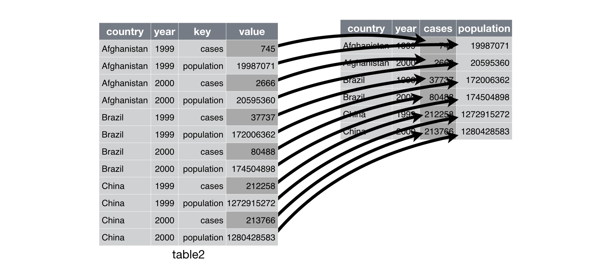
• Example table2 is not tidy (?). Actually this long format can be useful for plotting in ggplot2.

R

table2

# A tibble: 12 × 4
   country      year type            count
   <chr>       <int> <chr>           <int>
 1 Afghanistan  1999 cases             745
 2 Afghanistan  1999 population   19987071
 3 Afghanistan  2000 cases            2666
 4 Afghanistan  2000 population   20595360
 5 Brazil       1999 cases           37737
 6 Brazil       1999 population  172006362
 7 Brazil       2000 cases           80488
 8 Brazil       2000 population  174504898
 9 China        1999 cases          212258
10 China        1999 population 1272915272
11 China        2000 cases          213766
12 China        2000 population 1280428583

Python

table2 = pd.DataFrame({
    'country': ['Afghanistan', 'Afghanistan', 'Afghanistan', 'Afghanistan', 'Brazil', 'Brazil', 'Brazil', 'Brazil', 'China', 'China', 'China', 'China'],
    'year': [1999, 1999, 2000, 2000, 1999, 1999, 2000, 2000, 1999, 1999, 2000, 2000,],
    'type': ['cases', 'population', 'cases', 'population', 'cases', 'population', 'cases', 'population', 'cases', 'population', 'cases', 'population'],
    'count': [745, 19987071, 2666, 20595360, 37737, 172006362, 80488, 174504898, 212258, 1272915272, 213766, 1280428583]
})
table2

        country  year        type       count
0   Afghanistan  1999       cases         745
1   Afghanistan  1999  population    19987071
2   Afghanistan  2000       cases        2666
3   Afghanistan  2000  population    20595360
4        Brazil  1999       cases       37737
5        Brazil  1999  population   172006362
6        Brazil  2000       cases       80488
7        Brazil  2000  population   174504898
8         China  1999       cases      212258
9         China  1999  population  1272915272
10        China  2000       cases      213766
11        China  2000  population  1280428583

Julia

table2 = DataFrame(
    country = ["Afghanistan", "Afghanistan", "Afghanistan", "Afghanistan", "Brazil", "Brazil", "Brazil", "Brazil", "China", "China", "China", "China"],
    year = [1999, 1999, 2000, 2000, 1999, 1999, 2000, 2000, 1999, 1999, 2000, 2000,],
    type = ["cases", "population", "cases", "population", "cases", "population", "cases", "population", "cases", "population", "cases", "population"],
    count = [745, 19987071, 2666, 20595360, 37737, 172006362, 80488, 174504898, 212258, 1272915272, 213766, 1280428583]
)

12×4 DataFrame
 Row │ country      year   type        count
     │ String       Int64  String      Int64
─────┼────────────────────────────────────────────
   1 │ Afghanistan   1999  cases              745
   2 │ Afghanistan   1999  population    19987071
   3 │ Afghanistan   2000  cases             2666
   4 │ Afghanistan   2000  population    20595360
   5 │ Brazil        1999  cases            37737
   6 │ Brazil        1999  population   172006362
   7 │ Brazil        2000  cases            80488
   8 │ Brazil        2000  population   174504898
   9 │ China         1999  cases           212258
  10 │ China         1999  population  1272915272
  11 │ China         2000  cases           213766
  12 │ China         2000  population  1280428583

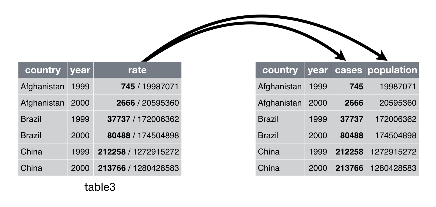
• Example table3 is not tidy.

R

table3

# A tibble: 6 × 3
  country      year rate             
* <chr>       <int> <chr>            
1 Afghanistan  1999 745/19987071     
2 Afghanistan  2000 2666/20595360    
3 Brazil       1999 37737/172006362  
4 Brazil       2000 80488/174504898  
5 China        1999 212258/1272915272
6 China        2000 213766/1280428583

Python

table3 = pd.DataFrame({
    'country': ['Afghanistan', 'Afghanistan', 'Brazil', 'Brazil', 'China', 'China'],
    'year': [1999, 2000, 1999, 2000, 1999, 2000],
    'rate': ['745/19987071', '2666/20595360', '37737/172006362', '80488/174504898', '212258/1272915272', '213766/1280428583']
})
table3

       country  year               rate
0  Afghanistan  1999       745/19987071
1  Afghanistan  2000      2666/20595360
2       Brazil  1999    37737/172006362
3       Brazil  2000    80488/174504898
4        China  1999  212258/1272915272
5        China  2000  213766/1280428583

Julia

table3 = DataFrame(
    country = ["Afghanistan", "Afghanistan", "Brazil", "Brazil", "China", "China"],
    year = [1999, 2000, 1999, 2000, 1999, 2000],
    rate = ["745/19987071", "2666/20595360", "37737/172006362", "80488/174504898", "212258/1272915272", "213766/1280428583"]
)

6×3 DataFrame
 Row │ country      year   rate
     │ String       Int64  String
─────┼───────────────────────────────────────
   1 │ Afghanistan   1999  745/19987071
   2 │ Afghanistan   2000  2666/20595360
   3 │ Brazil        1999  37737/172006362
   4 │ Brazil        2000  80488/174504898
   5 │ China         1999  212258/1272915272
   6 │ China         2000  213766/1280428583

• table4a and table4b are not tidy.

R

table4a

# A tibble: 3 × 3
  country     `1999` `2000`
* <chr>        <int>  <int>
1 Afghanistan    745   2666
2 Brazil       37737  80488
3 China       212258 213766

table4b

# A tibble: 3 × 3
  country         `1999`     `2000`
* <chr>            <int>      <int>
1 Afghanistan   19987071   20595360
2 Brazil       172006362  174504898
3 China       1272915272 1280428583

Python

table4a = pd.DataFrame({
    'country': ['Afghanistan', 'Brazil', 'China'],
    '1999': [745, 37737, 212258],
    '2000': [2666, 80488, 213766]
})
table4a

       country    1999    2000
0  Afghanistan     745    2666
1       Brazil   37737   80488
2        China  212258  213766

table4b = pd.DataFrame({
    'country': ['Afghanistan', 'Brazil', 'China'],
    '1999': [19987071, 172006362, 1272915272],
    '2000': [20595360, 174504898, 1280428583]
})
table4b

       country        1999        2000
0  Afghanistan    19987071    20595360
1       Brazil   172006362   174504898
2        China  1272915272  1280428583

Julia

table4a = DataFrame(
    country = ["Afghanistan", "Brazil", "China"],
    y1999 = [745, 37737, 212258],
    y2000 = [2666, 80488, 213766]
);
rename!(table4a, Dict(:y1999 => Symbol("1999"), :y2000 => Symbol("2000")))

3×3 DataFrame
 Row │ country      1999    2000
     │ String       Int64   Int64
─────┼─────────────────────────────
   1 │ Afghanistan     745    2666
   2 │ Brazil        37737   80488
   3 │ China        212258  213766

table4b = DataFrame(
    country = ["Afghanistan", "Brazil", "China"],
    y1999 = [19987071, 172006362, 1272915272],
    y2000 = [20595360, 174504898, 1280428583]
);
rename!(table4b, Dict(:y1999 => Symbol("1999"), :y2000 => Symbol("2000")))

3×3 DataFrame
 Row │ country      1999        2000
     │ String       Int64       Int64
─────┼─────────────────────────────────────
   1 │ Afghanistan    19987071    20595360
   2 │ Brazil        172006362   174504898
   3 │ China        1272915272  1280428583

5.2 pivot_longer (gathering)

• gather (deprecated command) columns into a new pair of variables.

# Deprecated command
table4a %>%
  gather(`1999`, `2000`, key = "year", value = "cases")

# A tibble: 6 × 3
  country     year   cases
  <chr>       <chr>  <int>
1 Afghanistan 1999     745
2 Brazil      1999   37737
3 China       1999  212258
4 Afghanistan 2000    2666
5 Brazil      2000   80488
6 China       2000  213766

• gather function has been superseded by pivot_longer.

• In Python, it’s called melt. In Julia, it’s called stack.

R

table4a %>%
  pivot_longer(c(`1999`, `2000`), names_to = "year", values_to = "cases")

# A tibble: 6 × 3
  country     year   cases
  <chr>       <chr>  <int>
1 Afghanistan 1999     745
2 Afghanistan 2000    2666
3 Brazil      1999   37737
4 Brazil      2000   80488
5 China       1999  212258
6 China       2000  213766

Python

tidy4a = table4a.melt(
  id_vars = ['country'],
  value_vars = ['1999', '2000'],
  var_name = 'year',
  value_name = 'cases'
)
tidy4a

       country  year   cases
0  Afghanistan  1999     745
1       Brazil  1999   37737
2        China  1999  212258
3  Afghanistan  2000    2666
4       Brazil  2000   80488
5        China  2000  213766

Julia

tidy4a = @pipe stack(table4a, ["1999", "2000"]) |> 
  rename!(_, Dict(:variable => :year, :value => :cases))

6×3 DataFrame
 Row │ country      year    cases
     │ String       String  Int64
─────┼─────────────────────────────
   1 │ Afghanistan  1999       745
   2 │ Brazil       1999     37737
   3 │ China        1999    212258
   4 │ Afghanistan  2000      2666
   5 │ Brazil       2000     80488
   6 │ China        2000    213766

• We can gather table4b too and then join them

R

tidy4a <- table4a %>% 
  pivot_longer(c(`1999`, `2000`), names_to = "year", values_to = "cases")
# gather(`1999`, `2000`, key = "year", value = "cases")
tidy4b <- table4b %>% 
  pivot_longer(c(`1999`, `2000`), names_to = "year", values_to = "population")
# gather(`1999`, `2000`, key = "year", value = "population")
left_join(tidy4a, tidy4b)

Joining, by = c("country", "year")

# A tibble: 6 × 4
  country     year   cases population
  <chr>       <chr>  <int>      <int>
1 Afghanistan 1999     745   19987071
2 Afghanistan 2000    2666   20595360
3 Brazil      1999   37737  172006362
4 Brazil      2000   80488  174504898
5 China       1999  212258 1272915272
6 China       2000  213766 1280428583

Python

tidy4b = table4b.melt(
    id_vars = ['country'],
    value_vars = ['1999', '2000'],
    var_name = 'year',
    value_name = 'population'
    )
tidy4b

       country  year  population
0  Afghanistan  1999    19987071
1       Brazil  1999   172006362
2        China  1999  1272915272
3  Afghanistan  2000    20595360
4       Brazil  2000   174504898
5        China  2000  1280428583

tidy4a.merge(
    tidy4b,
    on = ['country', 'year'],
    how = 'left'
    )

       country  year   cases  population
0  Afghanistan  1999     745    19987071
1       Brazil  1999   37737   172006362
2        China  1999  212258  1272915272
3  Afghanistan  2000    2666    20595360
4       Brazil  2000   80488   174504898
5        China  2000  213766  1280428583

Julia

tidy4b = @pipe stack(table4b, ["1999", "2000"]) |> rename!(_, Dict(:variable => :year, :value => :population))

6×3 DataFrame
 Row │ country      year    population
     │ String       String  Int64
─────┼─────────────────────────────────
   1 │ Afghanistan  1999      19987071
   2 │ Brazil       1999     172006362
   3 │ China        1999    1272915272
   4 │ Afghanistan  2000      20595360
   5 │ Brazil       2000     174504898
   6 │ China        2000    1280428583

leftjoin!(tidy4a, tidy4b, on = [:country, :year])

6×4 DataFrame
 Row │ country      year    cases   population
     │ String       String  Int64   Int64?
─────┼─────────────────────────────────────────
   1 │ Afghanistan  1999       745    19987071
   2 │ Brazil       1999     37737   172006362
   3 │ China        1999    212258  1272915272
   4 │ Afghanistan  2000      2666    20595360
   5 │ Brazil       2000     80488   174504898
   6 │ China        2000    213766  1280428583

5.3 pivot_wider (spreading)

• Spreading is the opposite of gathering.

table2 %>%
  spread(key = type, value = count)

# A tibble: 6 × 4
  country      year  cases population
  <chr>       <int>  <int>      <int>
1 Afghanistan  1999    745   19987071
2 Afghanistan  2000   2666   20595360
3 Brazil       1999  37737  172006362
4 Brazil       2000  80488  174504898
5 China        1999 212258 1272915272
6 China        2000 213766 1280428583

• spread function has been superseded by pivot_wider.

• In Python, it’s called pivot. In Julia, it’s called unstack.

R

table2 %>%
  pivot_wider(names_from = type, values_from = count)

# A tibble: 6 × 4
  country      year  cases population
  <chr>       <int>  <int>      <int>
1 Afghanistan  1999    745   19987071
2 Afghanistan  2000   2666   20595360
3 Brazil       1999  37737  172006362
4 Brazil       2000  80488  174504898
5 China        1999 212258 1272915272
6 China        2000 213766 1280428583

Python

table2.pivot(
    index = ['country', 'year'],
    columns = 'type',
    values = 'count'
)

type               cases  population
country     year                    
Afghanistan 1999     745    19987071
            2000    2666    20595360
Brazil      1999   37737   172006362
            2000   80488   174504898
China       1999  212258  1272915272
            2000  213766  1280428583

Julia

unstack(table2, :type, :count)

6×4 DataFrame
 Row │ country      year   cases   population
     │ String       Int64  Int64?  Int64?
─────┼────────────────────────────────────────
   1 │ Afghanistan   1999     745    19987071
   2 │ Afghanistan   2000    2666    20595360
   3 │ Brazil        1999   37737   172006362
   4 │ Brazil        2000   80488   174504898
   5 │ China         1999  212258  1272915272
   6 │ China         2000  213766  1280428583

5.4 Separating

R

# Before separation
table3

# A tibble: 6 × 3
  country      year rate             
* <chr>       <int> <chr>            
1 Afghanistan  1999 745/19987071     
2 Afghanistan  2000 2666/20595360    
3 Brazil       1999 37737/172006362  
4 Brazil       2000 80488/174504898  
5 China        1999 212258/1272915272
6 China        2000 213766/1280428583

# After separation
table3 %>% 
  separate(rate, into = c("cases", "population"))

# A tibble: 6 × 4
  country      year cases  population
  <chr>       <int> <chr>  <chr>     
1 Afghanistan  1999 745    19987071  
2 Afghanistan  2000 2666   20595360  
3 Brazil       1999 37737  172006362 
4 Brazil       2000 80488  174504898 
5 China        1999 212258 1272915272
6 China        2000 213766 1280428583

• Separate into numeric values:

table3 %>% 
  separate(rate, into = c("cases", "population"), convert = TRUE)

# A tibble: 6 × 4
  country      year  cases population
  <chr>       <int>  <int>      <int>
1 Afghanistan  1999    745   19987071
2 Afghanistan  2000   2666   20595360
3 Brazil       1999  37737  172006362
4 Brazil       2000  80488  174504898
5 China        1999 212258 1272915272
6 China        2000 213766 1280428583

• Separate at a fixed position:

table3 %>% 
  separate(year, into = c("century", "year"), sep = 2)

# A tibble: 6 × 4
  country     century year  rate             
  <chr>       <chr>   <chr> <chr>            
1 Afghanistan 19      99    745/19987071     
2 Afghanistan 20      00    2666/20595360    
3 Brazil      19      99    37737/172006362  
4 Brazil      20      00    80488/174504898  
5 China       19      99    212258/1272915272
6 China       20      00    213766/1280428583

Python

# Before separation
table3
# After separation

       country  year               rate
0  Afghanistan  1999       745/19987071
1  Afghanistan  2000      2666/20595360
2       Brazil  1999    37737/172006362
3       Brazil  2000    80488/174504898
4        China  1999  212258/1272915272
5        China  2000  213766/1280428583

table3[['cases', 'population']] = table3['rate'].apply(lambda x: pd.Series(str(x).split("/")))
table3

       country  year               rate   cases  population
0  Afghanistan  1999       745/19987071     745    19987071
1  Afghanistan  2000      2666/20595360    2666    20595360
2       Brazil  1999    37737/172006362   37737   172006362
3       Brazil  2000    80488/174504898   80488   174504898
4        China  1999  212258/1272915272  212258  1272915272
5        China  2000  213766/1280428583  213766  1280428583

Julia

using SplitApplyCombine

# Before separation
table3

6×3 DataFrame
 Row │ country      year   rate
     │ String       Int64  String
─────┼───────────────────────────────────────
   1 │ Afghanistan   1999  745/19987071
   2 │ Afghanistan   2000  2666/20595360
   3 │ Brazil        1999  37737/172006362
   4 │ Brazil        2000  80488/174504898
   5 │ China         1999  212258/1272915272
   6 │ China         2000  213766/1280428583

# After separation
insertcols!(table3, ([:cases, :population] .=> invert(split.(table3.rate, "/")))..., makeunique = true)

6×5 DataFrame
 Row │ country      year   rate               cases      population
     │ String       Int64  String             SubStrin…  SubStrin…
─────┼──────────────────────────────────────────────────────────────
   1 │ Afghanistan   1999  745/19987071       745        19987071
   2 │ Afghanistan   2000  2666/20595360      2666       20595360
   3 │ Brazil        1999  37737/172006362    37737      172006362
   4 │ Brazil        2000  80488/174504898    80488      174504898
   5 │ China         1999  212258/1272915272  212258     1272915272
   6 │ China         2000  213766/1280428583  213766     1280428583

5.5 Unite

R

# Before unite
table5

# A tibble: 6 × 4
  country     century year  rate             
* <chr>       <chr>   <chr> <chr>            
1 Afghanistan 19      99    745/19987071     
2 Afghanistan 20      00    2666/20595360    
3 Brazil      19      99    37737/172006362  
4 Brazil      20      00    80488/174504898  
5 China       19      99    212258/1272915272
6 China       20      00    213766/1280428583

• unite() is the inverse of separate().

# After unite
table5 %>% 
  unite(new, century, year, sep = "")

# A tibble: 6 × 3
  country     new   rate             
  <chr>       <chr> <chr>            
1 Afghanistan 1999  745/19987071     
2 Afghanistan 2000  2666/20595360    
3 Brazil      1999  37737/172006362  
4 Brazil      2000  80488/174504898  
5 China       1999  212258/1272915272
6 China       2000  213766/1280428583

Python

# Before unite
table5 = pd.DataFrame({
    'country': ['Afghanistan', 'Afghanistan', 'Brazil', 'Brazil', 'China', 'China'],
    'century': ['19', '20', '19', '20', '19', '20'],
    'year': ['99', '00', '99', '00', '99', '00'],
    'rate': ['745/19987071', '2666/20595360', '37737/172006362', '80488/174504898', '212258/1272915272', '213766/1280428583']
})
table5

       country century year               rate
0  Afghanistan      19   99       745/19987071
1  Afghanistan      20   00      2666/20595360
2       Brazil      19   99    37737/172006362
3       Brazil      20   00    80488/174504898
4        China      19   99  212258/1272915272
5        China      20   00  213766/1280428583

# After unite
table5['new'] = table5['century'] + table5['year']
table5

       country century year               rate   new
0  Afghanistan      19   99       745/19987071  1999
1  Afghanistan      20   00      2666/20595360  2000
2       Brazil      19   99    37737/172006362  1999
3       Brazil      20   00    80488/174504898  2000
4        China      19   99  212258/1272915272  1999
5        China      20   00  213766/1280428583  2000

Julia

# Before unite
table5 = DataFrame(
    country = ["Afghanistan", "Afghanistan", "Brazil", "Brazil", "China", "China"],
    century = ["19", "20", "19", "20", "19", "20"],
    year = ["99", "00", "99", "00", "99", "00"],
    rate = ["745/19987071", "2666/20595360", "37737/172006362", "80488/174504898", "212258/1272915272", "213766/1280428583"]
)

6×4 DataFrame
 Row │ country      century  year    rate
     │ String       String   String  String
─────┼─────────────────────────────────────────────────
   1 │ Afghanistan  19       99      745/19987071
   2 │ Afghanistan  20       00      2666/20595360
   3 │ Brazil       19       99      37737/172006362
   4 │ Brazil       20       00      80488/174504898
   5 │ China        19       99      212258/1272915272
   6 │ China        20       00      213766/1280428583

# After unite
table5[!, :new] = parse.(Int, string.(table5[!, :century]) .* string.(table5[!, :year]));
table5

6×5 DataFrame
 Row │ country      century  year    rate               new
     │ String       String   String  String             Int64
─────┼────────────────────────────────────────────────────────
   1 │ Afghanistan  19       99      745/19987071        1999
   2 │ Afghanistan  20       00      2666/20595360       2000
   3 │ Brazil       19       99      37737/172006362     1999
   4 │ Brazil       20       00      80488/174504898     2000
   5 │ China        19       99      212258/1272915272   1999
   6 │ China        20       00      213766/1280428583   2000

5.6 Drop missing values and/or duplicate rows

• Here’s a tibble with some missing values and duplicated rows:

R

df = tibble(
  country = c("Afghanistan", "Afghanistan", "Brazil", "China"),
  year = c(1999, 1999, 1999, NA),
  cases = c(745, 745, NA, 212258)
) %>% print()

# A tibble: 4 × 3
  country      year  cases
  <chr>       <dbl>  <dbl>
1 Afghanistan  1999    745
2 Afghanistan  1999    745
3 Brazil       1999     NA
4 China          NA 212258

Python

df = pd.DataFrame({
    'country': ["Afghanistan", "Afghanistan", "Brazil", "China"],
    'year': [1999, 1999, 1999, None],
    'cases': [745, 745, None, 212258]
})
df

       country    year     cases
0  Afghanistan  1999.0     745.0
1  Afghanistan  1999.0     745.0
2       Brazil  1999.0       NaN
3        China     NaN  212258.0

Julia

df = DataFrame(
    country = ["Afghanistan", "Afghanistan", "Brazil", "China"],
    year = [1999, 1999, 1999, missing],
    cases = [745, 745, missing, 212258]
)

4×3 DataFrame
 Row │ country      year     cases
     │ String       Int64?   Int64?
─────┼───────────────────────────────
   1 │ Afghanistan     1999      745
   2 │ Afghanistan     1999      745
   3 │ Brazil          1999  missing
   4 │ China        missing   212258

• To drop all rows with missing values

R

df %>% drop_na()

# A tibble: 2 × 3
  country      year cases
  <chr>       <dbl> <dbl>
1 Afghanistan  1999   745
2 Afghanistan  1999   745

Python

df.dropna()

       country    year  cases
0  Afghanistan  1999.0  745.0
1  Afghanistan  1999.0  745.0

Julia

dropmissing(df)

2×3 DataFrame
 Row │ country      year   cases
     │ String       Int64  Int64
─────┼───────────────────────────
   1 │ Afghanistan   1999    745
   2 │ Afghanistan   1999    745

• To remove duplicate rows

R

df %>%
  distinct()

# A tibble: 3 × 3
  country      year  cases
  <chr>       <dbl>  <dbl>
1 Afghanistan  1999    745
2 Brazil       1999     NA
3 China          NA 212258

Python

df.drop_duplicates()

       country    year     cases
0  Afghanistan  1999.0     745.0
2       Brazil  1999.0       NaN
3        China     NaN  212258.0

Julia

unique(df)

3×3 DataFrame
 Row │ country      year     cases
     │ String       Int64?   Int64?
─────┼───────────────────────────────
   1 │ Afghanistan     1999      745
   2 │ Brazil          1999  missing
   3 │ China        missing   212258