Display machine information for reproducibility.
R version 4.2.2 (2022-10-31)
Platform: x86_64-apple-darwin17.0 (64-bit)
Running under: macOS Big Sur ... 10.16

Matrix products: default
BLAS:   /Library/Frameworks/R.framework/Versions/4.2/Resources/lib/libRblas.0.dylib
LAPACK: /Library/Frameworks/R.framework/Versions/4.2/Resources/lib/libRlapack.dylib

locale:
[1] en_US.UTF-8/en_US.UTF-8/en_US.UTF-8/C/en_US.UTF-8/en_US.UTF-8

attached base packages:
[1] stats     graphics  grDevices utils     datasets  methods   base

other attached packages:
 [1] nycflights13_1.0.2 lubridate_1.9.0    timechange_0.1.1   forcats_0.5.2
 [5] stringr_1.5.0      dplyr_1.0.10       purrr_1.0.0        readr_2.1.3
 [9] tidyr_1.2.1        tibble_3.1.8       ggplot2_3.4.0      tidyverse_1.3.2

loaded via a namespace (and not attached):
 [1] tidyselect_1.2.0    xfun_0.35           haven_2.5.1
 [4] gargle_1.2.1        colorspace_2.0-3    vctrs_0.5.1
 [7] generics_0.1.3      htmltools_0.5.4     yaml_2.3.6
[10] utf8_1.2.2          rlang_1.0.6         pillar_1.8.1
[13] withr_2.5.0         glue_1.6.2          DBI_1.1.3
[16] dbplyr_2.2.1        modelr_0.1.10       readxl_1.4.1
[19] lifecycle_1.0.3     munsell_0.5.0       gtable_0.3.1
[22] cellranger_1.1.0    rvest_1.0.3         htmlwidgets_1.6.0
[25] evaluate_0.18       knitr_1.41          tzdb_0.3.0
[28] fastmap_1.1.0       fansi_1.0.3         broom_1.0.2
[31] backports_1.4.1     scales_1.2.1        googlesheets4_1.0.1
[34] jsonlite_1.8.4      fs_1.5.2            hms_1.1.2
[37] digest_0.6.30       stringi_1.7.8       grid_4.2.2
[40] cli_3.4.1           tools_4.2.2         magrittr_2.0.3
[43] crayon_1.5.2        pkgconfig_2.0.3     ellipsis_0.3.2
[46] xml2_1.3.3          reprex_2.0.2        googledrive_2.0.0
[49] assertthat_0.2.1    rmarkdown_2.18      httr_1.4.4
[52] rstudioapi_0.14     R6_2.5.1            compiler_4.2.2
import IPythonprint (IPython.sys_info())
{'commit_hash': 'add5877a4',
 'commit_source': 'installation',
 'default_encoding': 'utf-8',
 'ipython_path': '/Library/Frameworks/Python.framework/Versions/3.10/lib/python3.10/site-packages/IPython',
 'ipython_version': '8.8.0',
 'os_name': 'posix',
 'platform': 'macOS-10.16-x86_64-i386-64bit',
 'sys_executable': '/Library/Frameworks/Python.framework/Versions/3.10/bin/python3',
 'sys_platform': 'darwin',
 'sys_version': '3.10.9 (v3.10.9:1dd9be6584, Dec  6 2022, 14:37:36) [Clang '
                '13.0.0 (clang-1300.0.29.30)]'}
using InteractiveUtils versioninfo ()
Julia Version 1.8.3
Commit 0434deb161e (2022-11-14 20:14 UTC)
Platform Info:
  OS: macOS (x86_64-apple-darwin21.4.0)
  CPU: 8 × Intel(R) Core(TM) i7-6920HQ CPU @ 2.90GHz
  WORD_SIZE: 64
  LIBM: libopenlibm
  LLVM: libLLVM-13.0.1 (ORCJIT, skylake)
  Threads: 1 on 8 virtual cores
Environment:
  DYLD_FALLBACK_LIBRARY_PATH = /Library/Frameworks/R.framework/Resources/lib:/Library/Java/JavaVirtualMachines/jdk1.8.0_241.jdk/Contents/Home/jre/lib/server
  JULIA_EDITOR = code
Load tidyverse and lubridate (R), Pandas (Python), and DataFrames.jl (Julia).
library (lubridate)library (nycflights13)library (tidyverse)
# Load the pandas library import pandas as pd# Load numpy for array manipulation import numpy as np
using DataFrames , Pipe , StatsBase
Basics
Three types of data/time data:
date . Tibbles print it as <date>.time . Tibbles print it as <time>.date-time . Tibbles print it as <dttm>.
In the flights tibble, the last variable time_hour is in the data-time format:
%>% print (width = Inf )
# A tibble: 336,776 × 19
    year month   day dep_time sched_dep_time dep_delay arr_time sched_arr_time
   <int> <int> <int>    <int>          <int>     <dbl>    <int>          <int>
 1  2013     1     1      517            515         2      830            819
 2  2013     1     1      533            529         4      850            830
 3  2013     1     1      542            540         2      923            850
 4  2013     1     1      544            545        -1     1004           1022
 5  2013     1     1      554            600        -6      812            837
 6  2013     1     1      554            558        -4      740            728
 7  2013     1     1      555            600        -5      913            854
 8  2013     1     1      557            600        -3      709            723
 9  2013     1     1      557            600        -3      838            846
10  2013     1     1      558            600        -2      753            745
   arr_delay carrier flight tailnum origin dest  air_time distance  hour minute
       <dbl> <chr>    <int> <chr>   <chr>  <chr>    <dbl>    <dbl> <dbl>  <dbl>
 1        11 UA        1545 N14228  EWR    IAH        227     1400     5     15
 2        20 UA        1714 N24211  LGA    IAH        227     1416     5     29
 3        33 AA        1141 N619AA  JFK    MIA        160     1089     5     40
 4       -18 B6         725 N804JB  JFK    BQN        183     1576     5     45
 5       -25 DL         461 N668DN  LGA    ATL        116      762     6      0
 6        12 UA        1696 N39463  EWR    ORD        150      719     5     58
 7        19 B6         507 N516JB  EWR    FLL        158     1065     6      0
 8       -14 EV        5708 N829AS  LGA    IAD         53      229     6      0
 9        -8 B6          79 N593JB  JFK    MCO        140      944     6      0
10         8 AA         301 N3ALAA  LGA    ORD        138      733     6      0
   time_hour
   <dttm>
 1 2013-01-01 05:00:00
 2 2013-01-01 05:00:00
 3 2013-01-01 05:00:00
 4 2013-01-01 05:00:00
 5 2013-01-01 06:00:00
 6 2013-01-01 05:00:00
 7 2013-01-01 06:00:00
 8 2013-01-01 06:00:00
 9 2013-01-01 06:00:00
10 2013-01-01 06:00:00
# … with 336,766 more rows
The nycflights13 data is available from the nycflights13 package in Python.
from nycflights13 import flights
        year  month  day  ...  hour  minute             time_hour
0       2013      1    1  ...     5      15  2013-01-01T10:00:00Z
1       2013      1    1  ...     5      29  2013-01-01T10:00:00Z
2       2013      1    1  ...     5      40  2013-01-01T10:00:00Z
3       2013      1    1  ...     5      45  2013-01-01T10:00:00Z
4       2013      1    1  ...     6       0  2013-01-01T11:00:00Z
...      ...    ...  ...  ...   ...     ...                   ...
336771  2013      9   30  ...    14      55  2013-09-30T18:00:00Z
336772  2013      9   30  ...    22       0  2013-10-01T02:00:00Z
336773  2013      9   30  ...    12      10  2013-09-30T16:00:00Z
336774  2013      9   30  ...    11      59  2013-09-30T15:00:00Z
336775  2013      9   30  ...     8      40  2013-09-30T12:00:00Z

[336776 rows x 19 columns]
Note there are some differences of this flights data from that in tidyverse. The data types for some variables are different. There are no natural ways in Pandas to hold integer column with missing values; so dep_time , arr_time are float64 instead of int64.
<class 'pandas.core.frame.DataFrame'>
RangeIndex: 336776 entries, 0 to 336775
Data columns (total 19 columns):
 #   Column          Non-Null Count   Dtype
---  ------          --------------   -----
 0   year            336776 non-null  int64
 1   month           336776 non-null  int64
 2   day             336776 non-null  int64
 3   dep_time        328521 non-null  float64
 4   sched_dep_time  336776 non-null  int64
 5   dep_delay       328521 non-null  float64
 6   arr_time        328063 non-null  float64
 7   sched_arr_time  336776 non-null  int64
 8   arr_delay       327346 non-null  float64
 9   carrier         336776 non-null  object
 10  flight          336776 non-null  int64
 11  tailnum         334264 non-null  object
 12  origin          336776 non-null  object
 13  dest            336776 non-null  object
 14  air_time        327346 non-null  float64
 15  distance        336776 non-null  int64
 16  hour            336776 non-null  int64
 17  minute          336776 non-null  int64
 18  time_hour       336776 non-null  object
dtypes: float64(5), int64(9), object(5)
memory usage: 48.8+ MB
To be more consistent with nycflights13 in tidyverse, we cast time_hour to datetime type.
'time_hour' ] = pd.to_datetime(flights['time_hour' ])
Let’s use RCall.jl to retrieve the nycflights13 data from R.
using RCall """ library(nycflights13) """ = rcopy (R"flights" )
336776×19 DataFrame
    Row │ year   month  day    dep_time  sched_dep_time  dep_delay  arr_time   ⋯
        │ Int64  Int64  Int64  Int64?    Int64           Float64?   Int64?     ⋯
────────┼───────────────────────────────────────────────────────────────────────
      1 │  2013      1      1       517             515        2.0       830   ⋯
      2 │  2013      1      1       533             529        4.0       850
      3 │  2013      1      1       542             540        2.0       923
      4 │  2013      1      1       544             545       -1.0      1004
      5 │  2013      1      1       554             600       -6.0       812   ⋯
      6 │  2013      1      1       554             558       -4.0       740
      7 │  2013      1      1       555             600       -5.0       913
      8 │  2013      1      1       557             600       -3.0       709
   ⋮    │   ⋮      ⋮      ⋮       ⋮            ⋮             ⋮         ⋮       ⋱
 336770 │  2013      9     30      2349            2359      -10.0       325   ⋯
 336771 │  2013      9     30   missing            1842  missing     missing
 336772 │  2013      9     30   missing            1455  missing     missing
 336773 │  2013      9     30   missing            2200  missing     missing
 336774 │  2013      9     30   missing            1210  missing     missing   ⋯
 336775 │  2013      9     30   missing            1159  missing     missing
 336776 │  2013      9     30   missing             840  missing     missing
                                              12 columns and 336761 rows omitted
Create date/times
today and now
Today:
# current date-time now ()
[1] "2023-02-01 09:17:27 PST"
Today:
from datetime import date, datetime# Current date # Current date-time
datetime.date(2023, 2, 1)
datetime.datetime(2023, 2, 1, 17, 12, 30, 320526)
using Dates # Current date today ()# Current date-time now ()
From strings
ymd_hms ("2023-02-02 14:57:25" )
[1] "2023-02-02 14:57:25 UTC"
ymd_hm ("2023-02-02 14:57" )
[1] "2023-02-02 14:57:00 UTC"
from dateutil.parser import parse'2023-02-02' , '%Y-%m- %d ' ).date()# I have to use the package python-dateutils to parse Feb 2nd
datetime.date(2023, 2, 2)
'Feb 2nd, 2023' ).date()
datetime.date(2023, 2, 2)
'02-Feb-2023' , ' %d -%b-%Y' ).date()
datetime.date(2023, 2, 2)
'2023-02-02 14:57:25' , '%Y-%m- %d %H:%M:%S' )
datetime.datetime(2023, 2, 2, 14, 57, 25)
'2023-02-02 14:57' , '%Y-%m- %d %H:%M' )
datetime.datetime(2023, 2, 2, 14, 57)
Date ("2023-02-02" , dateformat"y-m-d" )# Not sure how to parse "Feb 2nd, 2023" ??? # Date("Feb 2nd, 2023", dateformat"u d, y") Date ("02-Feb-2023" , dateformat"d-u-y" )
DateTime ("2023-02-02 14:57:25" , dateformat"y-m-d H:M:S" )DateTime ("2023-02-02 14:57" , dateformat"y-m-d H:M" )
From unquoated numbers
2022 , 2 , 2 ).date()
datetime.date(2022, 2, 2)
From variables/columns in a tibble
%>% select (year, month, day, hour, minute) %>% mutate (departure = make_datetime (year, month, day, hour, minute))
# A tibble: 336,776 × 6
    year month   day  hour minute departure
   <int> <int> <int> <dbl>  <dbl> <dttm>
 1  2013     1     1     5     15 2013-01-01 05:15:00
 2  2013     1     1     5     29 2013-01-01 05:29:00
 3  2013     1     1     5     40 2013-01-01 05:40:00
 4  2013     1     1     5     45 2013-01-01 05:45:00
 5  2013     1     1     6      0 2013-01-01 06:00:00
 6  2013     1     1     5     58 2013-01-01 05:58:00
 7  2013     1     1     6      0 2013-01-01 06:00:00
 8  2013     1     1     6      0 2013-01-01 06:00:00
 9  2013     1     1     6      0 2013-01-01 06:00:00
10  2013     1     1     6      0 2013-01-01 06:00:00
# … with 336,766 more rows
<- function (year, month, day, time) {make_datetime (year, month, day, time %/% 100 , time %% 100 )<- flights %>% filter (! is.na (dep_time), ! is.na (arr_time)) %>% mutate (dep_time = make_datetime_100 (year, month, day, dep_time),arr_time = make_datetime_100 (year, month, day, arr_time),sched_dep_time = make_datetime_100 (year, month, day, sched_dep_time),sched_arr_time = make_datetime_100 (year, month, day, sched_arr_time)%>% select (origin, dest, ends_with ("delay" ), ends_with ("time" )) %>% print (width = Inf )
# A tibble: 328,063 × 9
   origin dest  dep_delay arr_delay dep_time            sched_dep_time
   <chr>  <chr>     <dbl>     <dbl> <dttm>              <dttm>
 1 EWR    IAH           2        11 2013-01-01 05:17:00 2013-01-01 05:15:00
 2 LGA    IAH           4        20 2013-01-01 05:33:00 2013-01-01 05:29:00
 3 JFK    MIA           2        33 2013-01-01 05:42:00 2013-01-01 05:40:00
 4 JFK    BQN          -1       -18 2013-01-01 05:44:00 2013-01-01 05:45:00
 5 LGA    ATL          -6       -25 2013-01-01 05:54:00 2013-01-01 06:00:00
 6 EWR    ORD          -4        12 2013-01-01 05:54:00 2013-01-01 05:58:00
 7 EWR    FLL          -5        19 2013-01-01 05:55:00 2013-01-01 06:00:00
 8 LGA    IAD          -3       -14 2013-01-01 05:57:00 2013-01-01 06:00:00
 9 JFK    MCO          -3        -8 2013-01-01 05:57:00 2013-01-01 06:00:00
10 LGA    ORD          -2         8 2013-01-01 05:58:00 2013-01-01 06:00:00
   arr_time            sched_arr_time      air_time
   <dttm>              <dttm>                 <dbl>
 1 2013-01-01 08:30:00 2013-01-01 08:19:00      227
 2 2013-01-01 08:50:00 2013-01-01 08:30:00      227
 3 2013-01-01 09:23:00 2013-01-01 08:50:00      160
 4 2013-01-01 10:04:00 2013-01-01 10:22:00      183
 5 2013-01-01 08:12:00 2013-01-01 08:37:00      116
 6 2013-01-01 07:40:00 2013-01-01 07:28:00      150
 7 2013-01-01 09:13:00 2013-01-01 08:54:00      158
 8 2013-01-01 07:09:00 2013-01-01 07:23:00       53
 9 2013-01-01 08:38:00 2013-01-01 08:46:00      140
10 2013-01-01 07:53:00 2013-01-01 07:45:00      138
# … with 328,053 more rows
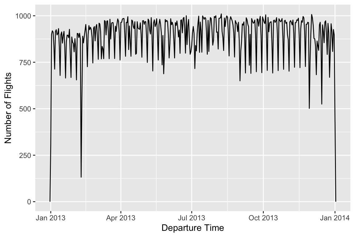
Now we can visualize the distribution of departure times across the year
%>% ggplot (aes (x= dep_time)) + geom_freqpoly (binwidth = 86400 ) + # 86400 seconds = 1 day labs (x = "Departure Time" ,y = "Number of Flights"
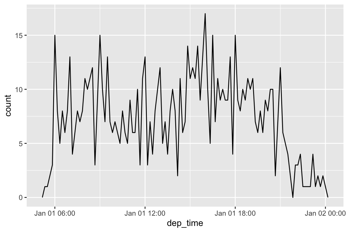
or within a single day:
%>% filter (dep_time < ymd (20130102 )) %>% ggplot (aes (dep_time)) + geom_freqpoly (binwidth = 600 ) # 600 s = 10 minutes
Getting components
<- ymd_hms ("2023-02-02 15:34:56" )year (datetime)
More information in month() and wday():
month (datetime, label = TRUE , abbr = FALSE )
[1] January
12 Levels: January < February < March < April < May < June < ... < December
wday (datetime, label = TRUE , abbr = FALSE )
[1] Thursday
7 Levels: Sunday < Monday < Tuesday < Wednesday < Thursday < ... < Saturday
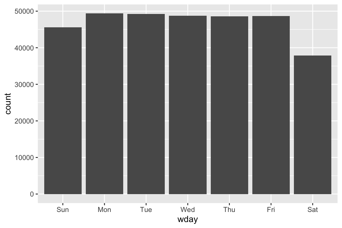
Visualize number of departures during a week:
%>% mutate (wday = wday (dep_time, label = TRUE )) %>% ggplot (aes (x = wday)) + geom_bar ()
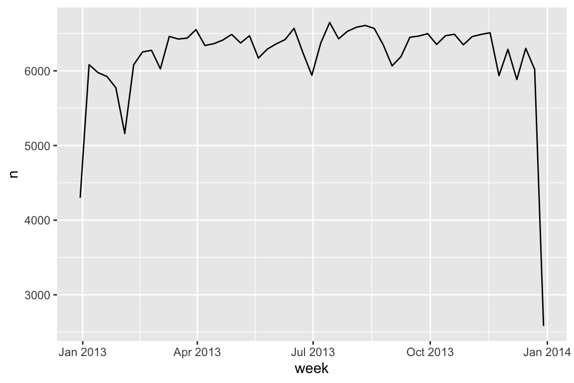
Rounding
floor_date(), round_date(), ceiling_date():
%>% count (week = floor_date (dep_time, "week" )) %>% ggplot (aes (x = week, y = n)) + geom_line ()
Time spans
Durations
Substract two dates we get a difftime object:
# How old is Hadley? <- today () - ymd (19791014 )
Time difference of 15816 days
lubridate provides the duration object that always uses seconds:
[1] "1366502400s (~43.3 years)"
Constructors for duration:
[1] "43200s (~12 hours)" "86400s (~1 days)"
[1] "0s"                "86400s (~1 days)"  "172800s (~2 days)"
[4] "259200s (~3 days)" "345600s (~4 days)" "432000s (~5 days)"
[1] "1814400s (~3 weeks)"
[1] "31557600s (~1 years)"
Periods
Durations represent an exact number of seconds:
<- ymd_hms ("2016-03-12 13:00:00" , tz = "America/New_York" )
[1] "2016-03-12 13:00:00 EST"
[1] "2016-03-13 14:00:00 EDT"
Periods are time spans but don’t have a fixed length in seconds, instead they work with “human” times, like days and months.
[1] "2016-03-12 13:00:00 EST"
[1] "2016-03-13 13:00:00 EDT"
Constructors for period:
[1] "12H 0M 0S" "24H 0M 0S"
[1] "1m 0d 0H 0M 0S" "2m 0d 0H 0M 0S" "3m 0d 0H 0M 0S" "4m 0d 0H 0M 0S"
[5] "5m 0d 0H 0M 0S" "6m 0d 0H 0M 0S"
Some planes appear to have arrived at their destination before they departed from New York City.
%>% filter (arr_time < dep_time) %>% print (width = Inf )
# A tibble: 10,640 × 9
   origin dest  dep_delay arr_delay dep_time            sched_dep_time
   <chr>  <chr>     <dbl>     <dbl> <dttm>              <dttm>
 1 EWR    BQN           9        -4 2013-01-01 19:29:00 2013-01-01 19:20:00
 2 JFK    DFW          59        NA 2013-01-01 19:39:00 2013-01-01 18:40:00
 3 EWR    TPA          -2         9 2013-01-01 20:58:00 2013-01-01 21:00:00
 4 EWR    SJU          -6       -12 2013-01-01 21:02:00 2013-01-01 21:08:00
 5 EWR    SFO          11       -14 2013-01-01 21:08:00 2013-01-01 20:57:00
 6 LGA    FLL         -10        -2 2013-01-01 21:20:00 2013-01-01 21:30:00
 7 EWR    MCO          41        43 2013-01-01 21:21:00 2013-01-01 20:40:00
 8 JFK    LAX          -7       -24 2013-01-01 21:28:00 2013-01-01 21:35:00
 9 EWR    FLL          49        28 2013-01-01 21:34:00 2013-01-01 20:45:00
10 EWR    FLL          -9       -14 2013-01-01 21:36:00 2013-01-01 21:45:00
   arr_time            sched_arr_time      air_time
   <dttm>              <dttm>                 <dbl>
 1 2013-01-01 00:03:00 2013-01-01 00:07:00      192
 2 2013-01-01 00:29:00 2013-01-01 21:51:00       NA
 3 2013-01-01 00:08:00 2013-01-01 23:59:00      159
 4 2013-01-01 01:46:00 2013-01-01 01:58:00      199
 5 2013-01-01 00:25:00 2013-01-01 00:39:00      354
 6 2013-01-01 00:16:00 2013-01-01 00:18:00      160
 7 2013-01-01 00:06:00 2013-01-01 23:23:00      143
 8 2013-01-01 00:26:00 2013-01-01 00:50:00      338
 9 2013-01-01 00:20:00 2013-01-01 23:52:00      152
10 2013-01-01 00:25:00 2013-01-01 00:39:00      154
# … with 10,630 more rows
These are the overnight flights. Let’s fix this:
<- flights_dt %>% mutate (overnight = arr_time < dep_time,arr_time = arr_time + days (overnight * 1 ),sched_arr_time = sched_arr_time + days (overnight * 1 )%>% print (width = Inf )
# A tibble: 328,063 × 10
   origin dest  dep_delay arr_delay dep_time            sched_dep_time
   <chr>  <chr>     <dbl>     <dbl> <dttm>              <dttm>
 1 EWR    IAH           2        11 2013-01-01 05:17:00 2013-01-01 05:15:00
 2 LGA    IAH           4        20 2013-01-01 05:33:00 2013-01-01 05:29:00
 3 JFK    MIA           2        33 2013-01-01 05:42:00 2013-01-01 05:40:00
 4 JFK    BQN          -1       -18 2013-01-01 05:44:00 2013-01-01 05:45:00
 5 LGA    ATL          -6       -25 2013-01-01 05:54:00 2013-01-01 06:00:00
 6 EWR    ORD          -4        12 2013-01-01 05:54:00 2013-01-01 05:58:00
 7 EWR    FLL          -5        19 2013-01-01 05:55:00 2013-01-01 06:00:00
 8 LGA    IAD          -3       -14 2013-01-01 05:57:00 2013-01-01 06:00:00
 9 JFK    MCO          -3        -8 2013-01-01 05:57:00 2013-01-01 06:00:00
10 LGA    ORD          -2         8 2013-01-01 05:58:00 2013-01-01 06:00:00
   arr_time            sched_arr_time      air_time overnight
   <dttm>              <dttm>                 <dbl> <lgl>
 1 2013-01-01 08:30:00 2013-01-01 08:19:00      227 FALSE
 2 2013-01-01 08:50:00 2013-01-01 08:30:00      227 FALSE
 3 2013-01-01 09:23:00 2013-01-01 08:50:00      160 FALSE
 4 2013-01-01 10:04:00 2013-01-01 10:22:00      183 FALSE
 5 2013-01-01 08:12:00 2013-01-01 08:37:00      116 FALSE
 6 2013-01-01 07:40:00 2013-01-01 07:28:00      150 FALSE
 7 2013-01-01 09:13:00 2013-01-01 08:54:00      158 FALSE
 8 2013-01-01 07:09:00 2013-01-01 07:23:00       53 FALSE
 9 2013-01-01 08:38:00 2013-01-01 08:46:00      140 FALSE
10 2013-01-01 07:53:00 2013-01-01 07:45:00      138 FALSE
# … with 328,053 more rows
Intervals
Intervals are time spans bound by two real date-times. Intervals can be accurately converted to periods and durations.
interval (ymd_hms ("2009-08-09 13:01:30" ), ymd_hms ("2009-08-09 12:00:00" ))
[1] 2009-08-09 13:01:30 UTC--2009-08-09 12:00:00 UTC
<- ymd_hms ("2009-03-08 01:59:59" ) # DST boundary <- ymd_hms ("2000-02-29 12:00:00" )<- date2 %--% dateas.duration (span)
[1] "284651999s (~9.02 years)"
[1] "9y 0m 7d 13H 59M 59S"