Neural Network and Deep Learning
Biostat 203B
Credit: This note heavily uses material from
An Introduction to Statistical Learning: with Applications in R (ISL2).
Elements of Statistical Learning: Data Mining, Inference, and Prediction (ESL2).
Stanford CS231n: http://cs231n.github.io.
On the origin of deep learning by Wang and Raj (2017): https://arxiv.org/pdf/1702.07800.pdf
Learning Deep Learning lectures by Dr. Qiyang Hu (UCLA Office of Advanced Research Computing): https://github.com/huqy/deep_learning_workshops
1 Overview
Neural networks became popular in the 1980s.
Lots of successes, hype, and great conferences: NeurIPS, Snowbird.
Then along came SVMs, Random Forests and Boosting in the 1990s, and Neural Networks took a back seat.
Re-emerged around 2010 as Deep Learning. By 2020s very dominant and successful.
Part of success due to vast improvements in computing power, larger training sets, and software: Tensorflow and PyTorch.
Much of the credit goes to three pioneers and their students: Yann LeCun, Geoffrey Hinton, and Yoshua Bengio, who received the 2018 ACM Turing Award for their work in Neural Networks.
2 History and recent surge
From Wang and Raj (2017):
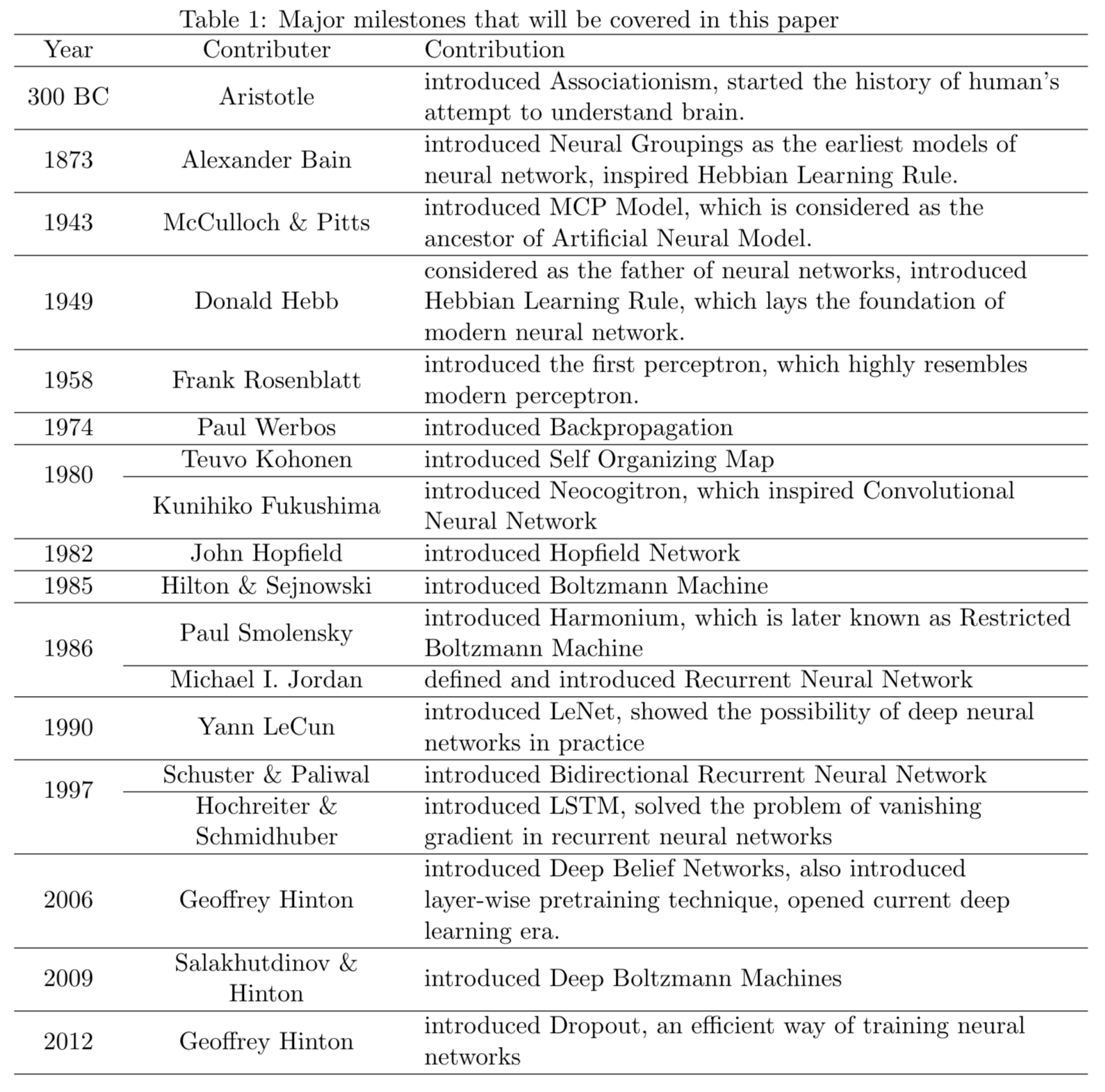
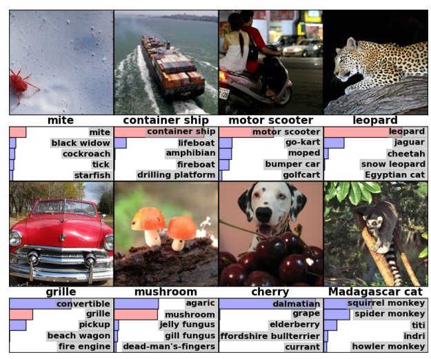
The current AI wave came in 2012 when AlexNet (60 million parameters) cuts the error rate of ImageNet competition (classify 1.2 million natural images) by half.
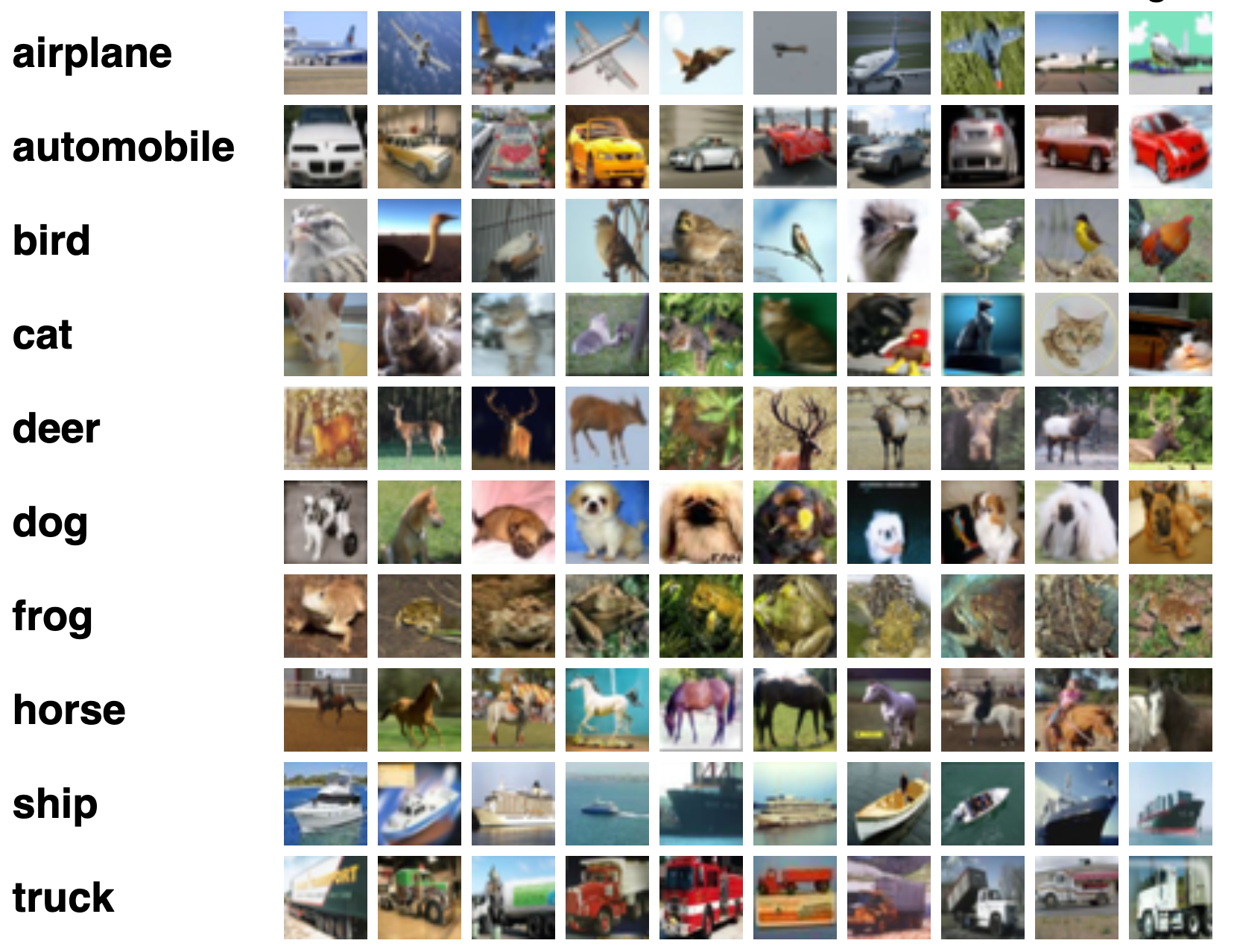
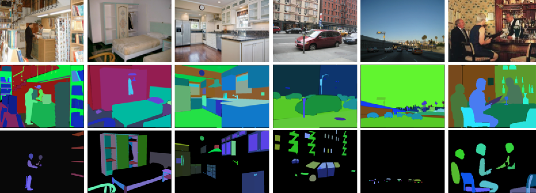
3 Canonical datasets for computer vision tasks
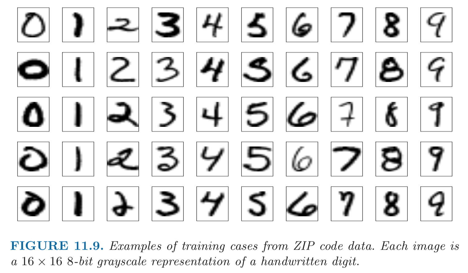
![]()
- Microsoft COCO (object detection, segmentation, and captioning)

- ADE20K (scene parsing)
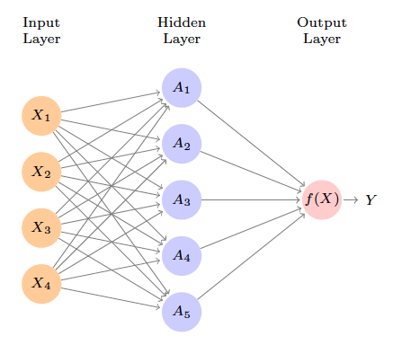
4 Single layer neural network
- Inspired by the biological neuron model.
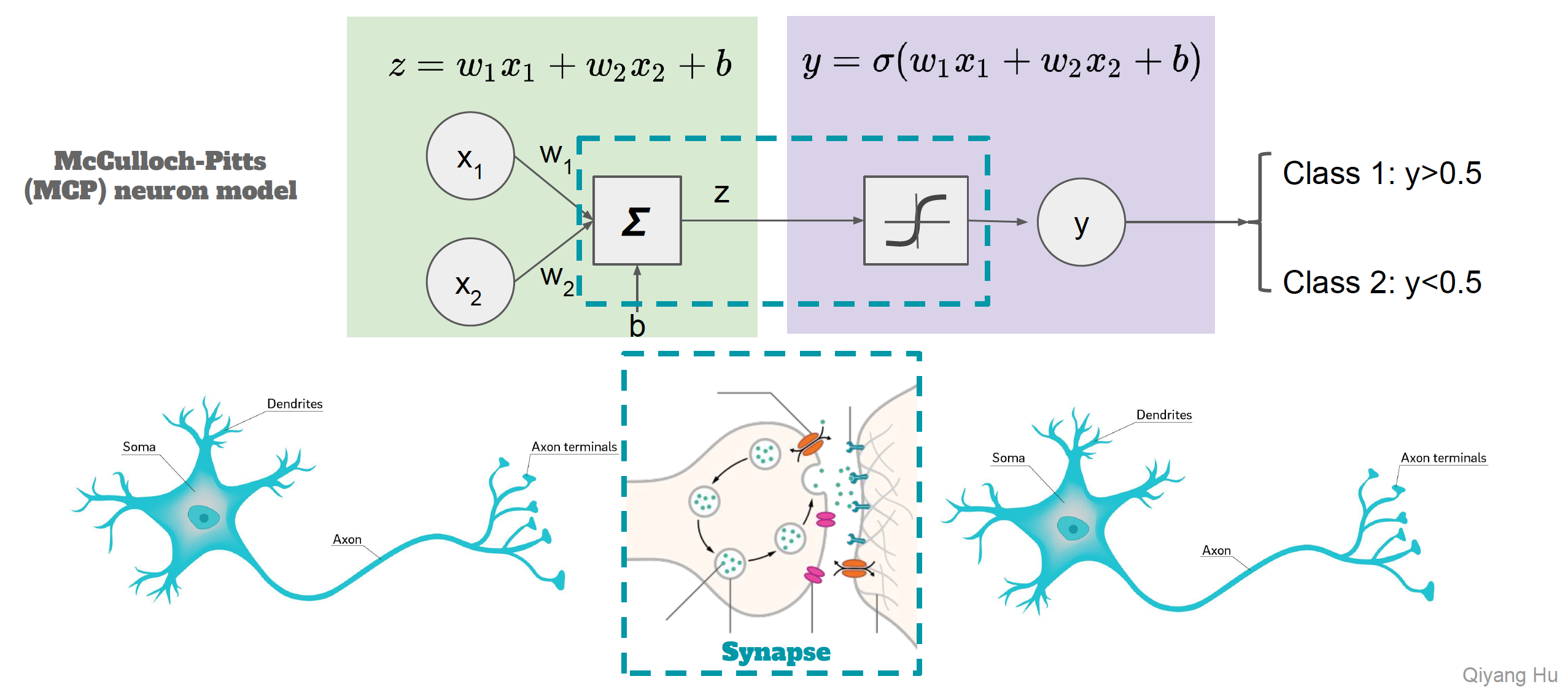
- Model:
\[\begin{eqnarray*} f(X) &=& \beta_0 + \sum_{k=1}^K \beta_k h_k(X) \\ &=& \beta_0 + \sum_{k=1}^K \beta_k g(w_{k0} + \sum_{j=1}^p w_{kj} X_j). \end{eqnarray*}\]
4.1 Activation functions
Activations in the hidden layer: \[ A_k = h_k(X) = g(w_{k0} + \sum_{j=1}^p w_{kj} X_j) \]
\(g(z)\) is called the activation function. Popular are the sigmoid and rectified linear, shown in figure.
Sigmoid activation: \[ g(z) = \frac{e^z}{1 + e^z} = \frac{1}{1 + e^{-z}}. \]
ReLU (rectified linear unit): \[ g(z) = (z)_+ = \begin{cases} 0 & \text{if } z<0 \\ z & \text{otherwise} \end{cases}. \] According to Wikipedia: The rectifier is, as of 2017, the most popular activation function for deep neural networks.
Activation functions in hidden layers are typically nonlinear, otherwise the model collapses to a linear model.
So the activations are like derived features. Nonlinear transformations of linear combinations of the features.
Consider a simple example with 2 input variables \(X=(X_1,X_2)\) and \(K=2\) hidden units \(h_1(X)\) and \(h_2(X)\) with \(g(z) = z^2\). Assumings specific parameter values \[\begin{eqnarray*} \beta_0 = 0, \beta_1 &=& \frac 14, \beta_2 = - \frac 14 \\ w_{10} = 0, w_{11} &=& 1, w_{12} = 1 \\ w_{20} = 0, w_{21} &=& 1, w_{22} = -1. \end{eqnarray*}\] Then \[\begin{eqnarray*} h_1(X) &=& (0 + X_1 + X_2)^2, \\ h_2(X) &=& (0 + X_1 - X_2)^2. \end{eqnarray*}\] Plugging, we get \[\begin{eqnarray*} f(X) &=& 0 + \frac 14 \cdot (0 + X_1 + X_2)^2 - \frac 14 \cdot (0 + X_1 - X_2)^2 \\ &=& \frac 14[(X_1 + X_2)^2 - (X_1 - X_2)^2] \\ &=& X_1 X_2. \end{eqnarray*}\] So the sum of two nonlinear transformations of linear functions can give us an interaction!
4.2 Loss function
- The model is fit by minimizing \[ \sum_{i=1}^n (y_{i} - f(x_i))^2. \] for regression.
5 Multiple layer neural network
Example: MNIST digits. Handwritten digits \(28 \times 28\) grayscale images. 60K train, 10K test images. Features are the 784 pixel grayscale values in [0,255]. Labels are the digit class 0-9.
Goal: build a classifier to predict the image class.
We build a two-layer network with 256 units at first layer, 128 units at second layer, and 10 units at output layer.
Along with intercepts (called biases) there are 235,146 parameters (referred to as weights).
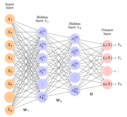
Output layer: Let \[ Z_m = \beta_{m0} + \sum_{\ell=1}^{K_2} \beta_{m\ell} A_{\ell}^{(2)}, m = 0,1,\ldots,9 \] be 10 linear combinations of activations at second layer.
Output activation function encodes the softmax function \[ f_m(X) = \operatorname{Pr}(Y = m \mid X) = \frac{e^{Z_m}}{\sum_{\ell=0}^9 e^{Z_{\ell}}}. \]
We fit the model by minimizing the negative multinomial log-likelihood (or cross-entropy): \[ \, - \sum_{i=1}^n \sum_{m=0}^9 y_{im} \log (f_m(x_i)). \] \(y_{im}=1\) if true class for observation \(i\) is \(m\), else 0 (one-hot encoded).
Results:
| Method | Test Error |
|---|---|
| Neural Network + Ridge Regularization | 2.3% |
| Neural Network + Dropout Regularization | 1.8% |
| Multinomial Logistic Regression | 7.2% |
| Linear Discriminant Analysis | 12.7% |
Early success for neural networks in the 1990s.
With so many parameters, regularization is essential.
Very overworked problem – best reported rates are <0.5%!
Human error rate is reported to be around 0.2%, or 20 of the 10K test images.
6 Expressivity of neural network
Playground: http://playground.tensorflow.org
Sources:
Consider the function \(F: \mathbb{R}^m \mapsto \mathbb{R}^n\) \[ F(\mathbf{v}) = \text{ReLU}(\mathbf{A} \mathbf{v} + \mathbf{b}). \] Each equation \[ \mathbf{a}_i^T \mathbf{v} + b_i = 0 \] creates a hyperplane in \(\mathbb{R}^m\). ReLU creates a fold along that hyperplane. There are a total of \(n\) folds.
- When there are \(n=2\) hyperplanes in \(\mathbb{R}^2\), 2 folds create 4 pieces.
- When there are \(n=3\) hyperplanes in \(\mathbb{R}^2\), 3 folds create 7 pieces.
- When there are \(n=2\) hyperplanes in \(\mathbb{R}^2\), 2 folds create 4 pieces.
The number of linear pieces of \(\mathbb{R}^m\) sliced by \(n\) hyperplanes is \[ r(n, m) = \sum_{i=0}^m \binom{n}{i} = \binom{n}{0} + \cdots + \binom{n}{m}. \]
Proof: Induction using the recursion \[ r(n, m) = r(n-1, m) + r(n-1, m-1). \]
Corollary:
- When there are relatively few neurons \(n \ll m\), \[ r(n,m) \approx 2^n. \]
- When there are many neurons \(n \gg m\), \[ r(n,m) \approx \frac{n^m}{m!}. \]
Counting the number of flat pieces with more hidden layers is much harder.
7 Universal approximation properties
Boolean Approximation: an MLP of one hidden layer can represent any Boolean function exactly.
Continuous Approximation: an MLP of one hidden layer can approximate any bounded continuous function with arbitrary accuracy.
Arbitrary Approximation: an MLP of two hidden layers can approximate any function with arbitrary accuracy.
8 Convolutional neural network (CNN)
- Major success story for classifying images.
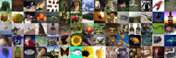
CIFAR100: 50K training images, 10K test images.
Each image is a three-dimensional array or feature map: \(32 \times 32 \times 3\) array of 8-bit numbers. The last dimension represents the three color channels for red, green and blue.
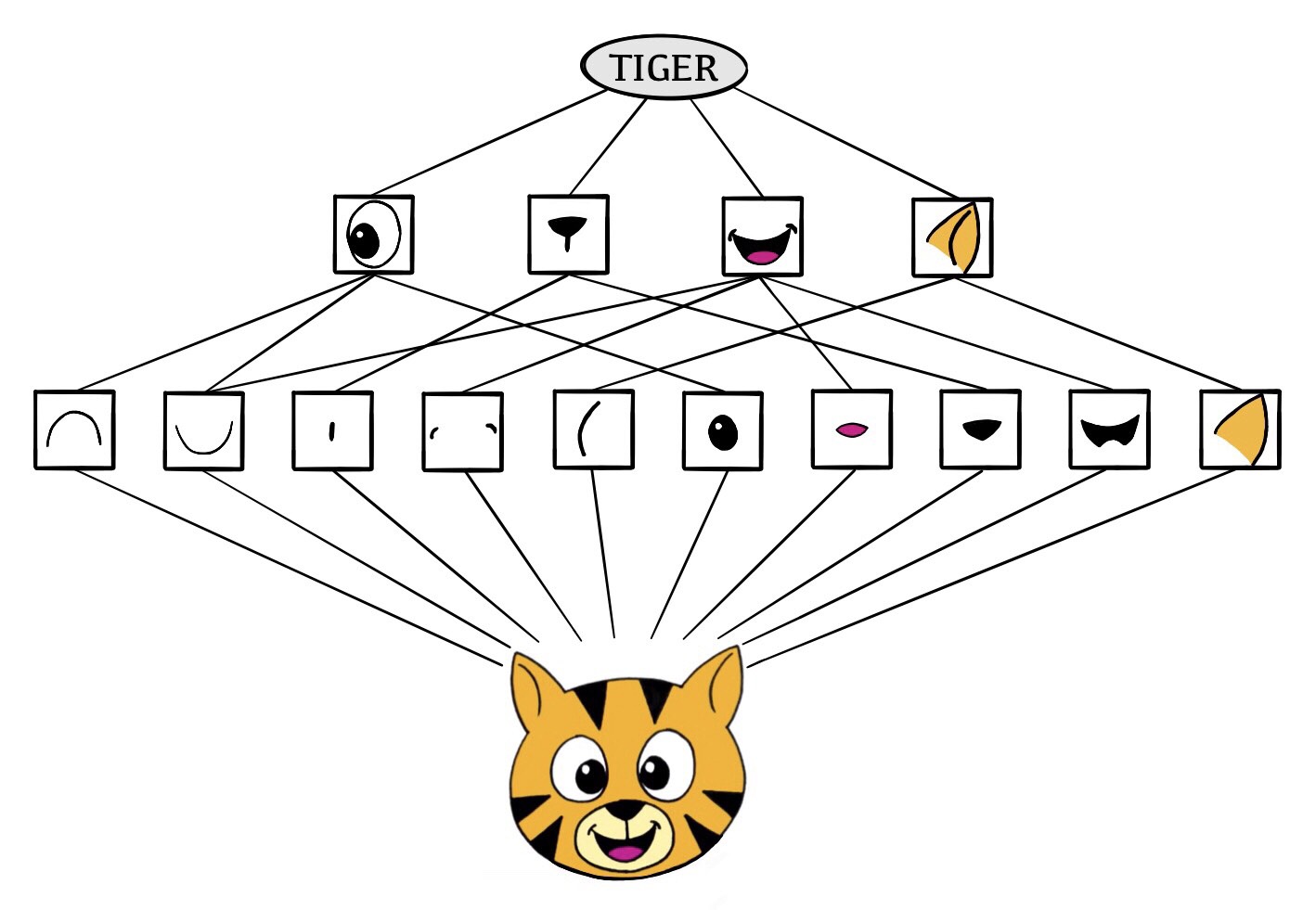
The CNN builds up an image in a hierarchical fashion.
Edges and shapes are recognized and pieced together to form more complex shapes, eventually assembling the target image.
This hierarchical construction is achieved using convolution and pooling layers.
8.1 Convolution
The convolution filter is itself an image, and represents a small shape, edge, etc.
We slide it around the input image, scoring for matches.
The scoring is done via dot-products, illustrated above. \[ \text{Input image} = \begin{pmatrix} a & b & c \\ d & e & f \\ g & h & i \\ j & k & l \end{pmatrix} \] \[ \text{Convolution Filter} = \begin{pmatrix} \alpha & \beta \\ \gamma & \delta \end{pmatrix} \] \[ \text{Convolved Image} = \begin{pmatrix} a \alpha + b \beta + d \gamma + e \delta & b \alpha + c \beta + e \gamma + f \delta \\ d \alpha + e \beta + g \gamma + h \delta & e \alpha + f \beta + h \gamma + i \delta \\ g \alpha + h \beta + j \gamma + k \delta & h \alpha + i \beta + k \gamma + l \delta \end{pmatrix} \]
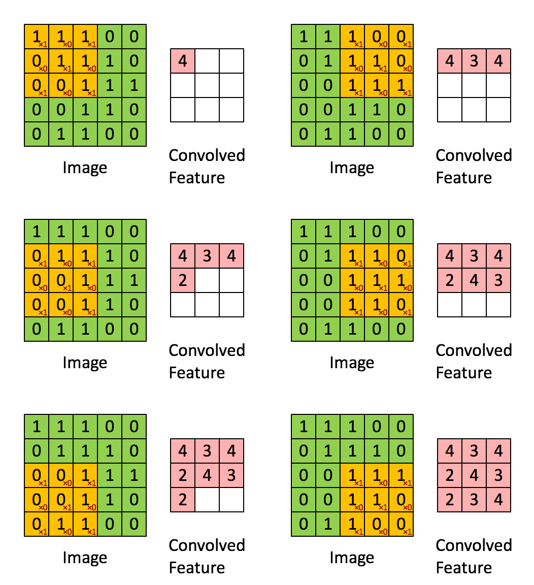
- If the subimage of the input image is similar to the filter, the score is high, otherwise low.
Interactive visualization: https://setosa.io/ev/image-kernels/
The filters are learned during training.
The idea of convolution with a filter is to find common patterns that occur in different parts of the image.
The result of the convolution is a new feature map.
Since images have three colors channels, the filter does as well: one filter per channel, and dot-products are summed.
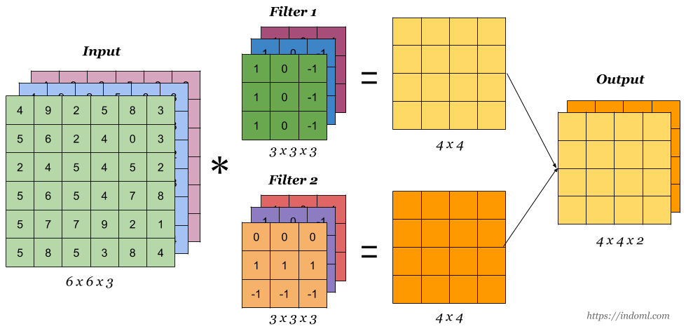
Source: https://indoml.com/2018/03/07/student-notes-convolutional-neural-networks-cnn-introduction/
8.2 Pooling
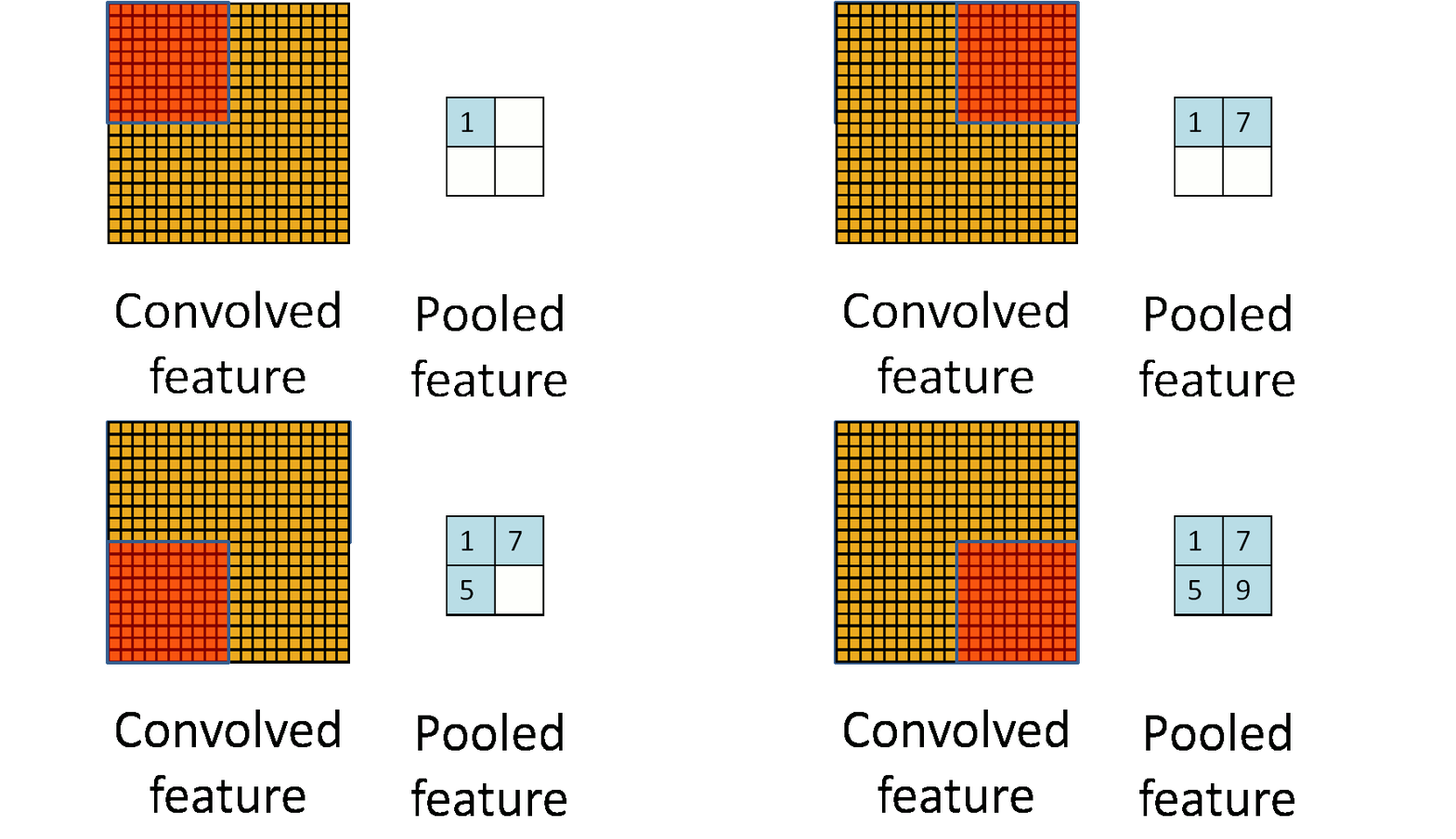
Max pool: \[ \begin{pmatrix} 1 & 2 & 5 & 3 \\ 3 & 0 & 1 & 2 \\ 2 & 1 & 3 & 4 \\ 1 & 1 & 2 & 0 \end{pmatrix} \to \begin{pmatrix} 3 & 5 \\ 2 & 4 \end{pmatrix} \]
Each non-overlapping \(2 \times 2\) block is replaced by its maximum.
This sharpens the feature identification.
Allows for locational invariance.
Reduces the dimension by a factor of 4.
8.3 CNN architecture
Many convolve + pool layers.
Filters are typically small, e.g. each channel \(3 \times 3\).
Each filter creates a new channel in convolution layer.
As pooling reduces size, the number of filters/channels is typically increased.
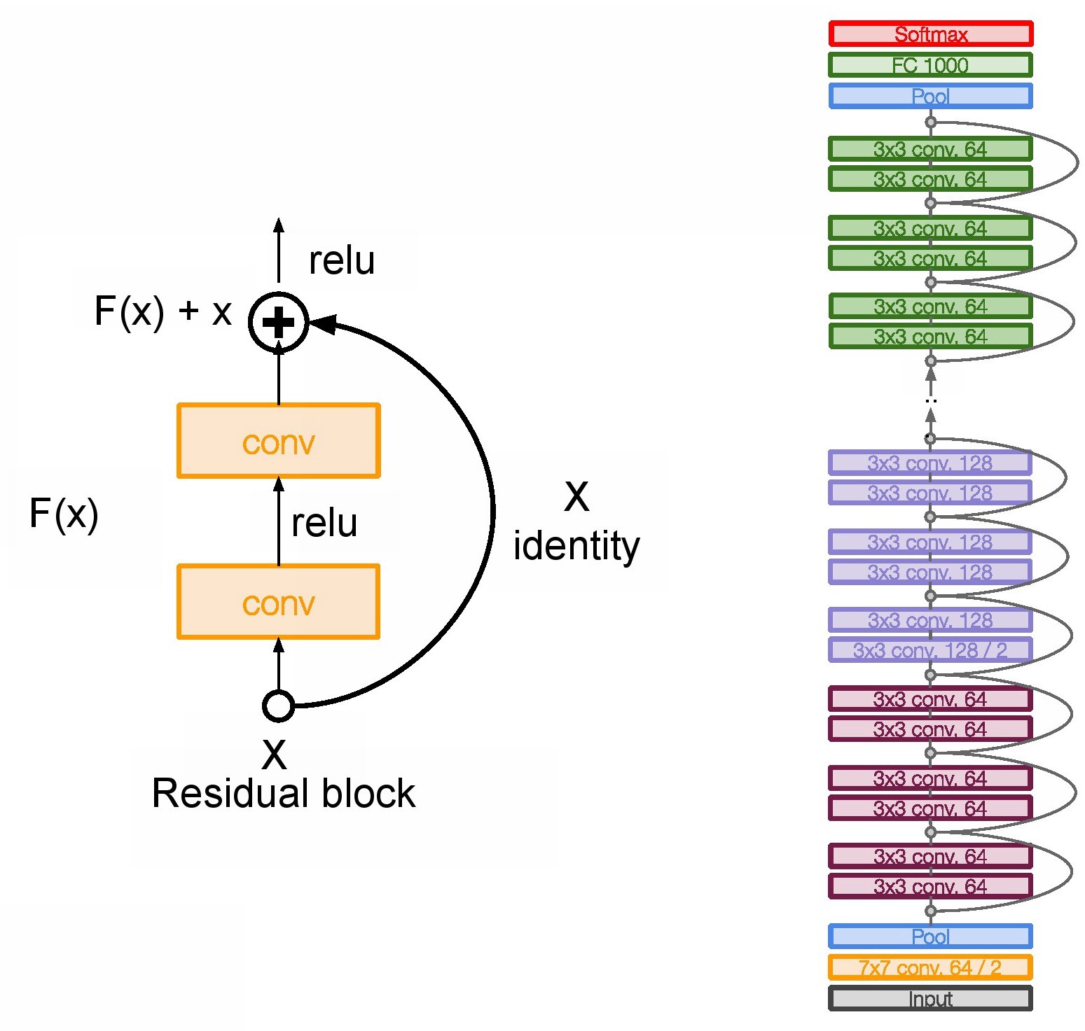
Number of layers can be very large. E.g. resnet50 trained on ImageNet 1000-class image data base has 50 layers!
8.4 Results using pre-trained resnet50
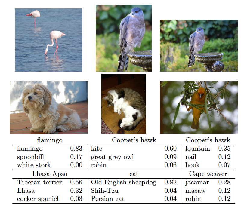
9 Popular architectures for image classification
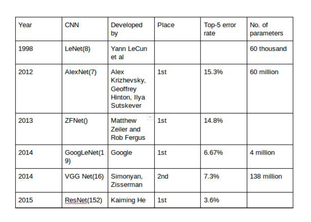
Source: Architecture comparison of AlexNet, VGGNet, ResNet, Inception, DenseNet
9.1 AlexNet
Source: http://cs231n.github.io/convolutional-networks/
ImageNet dataset. Classify 1.2 million high-resolution images (\(224 \times 224 \times 3\)) into 1000 classes.
AlexNet: Krizhevsky, Sutskever, Hinton (2012)
A combination of techniques: GPU, ReLU, DropOut (0.5), SGD + Momentum with 0.9, initial learning rate 0.01 and again reduced by 10 when validation accuracy become flat.
5 convolutional layers, pooling interspersed, 3 fully connected layers. \(\sim 60\) million parameters, 650,000 neurons.
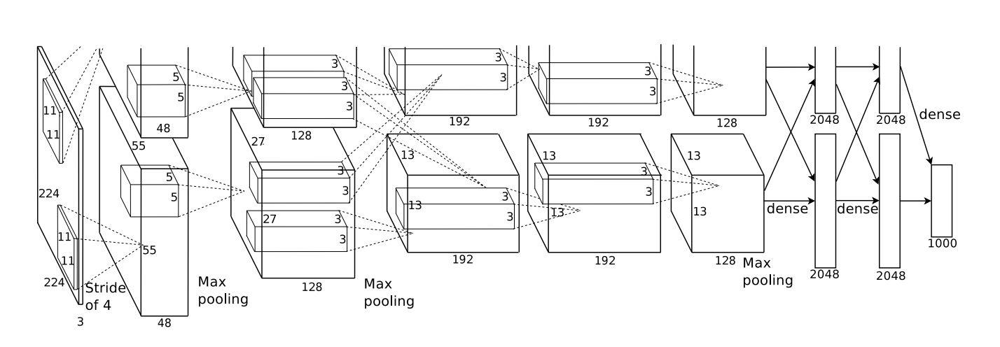
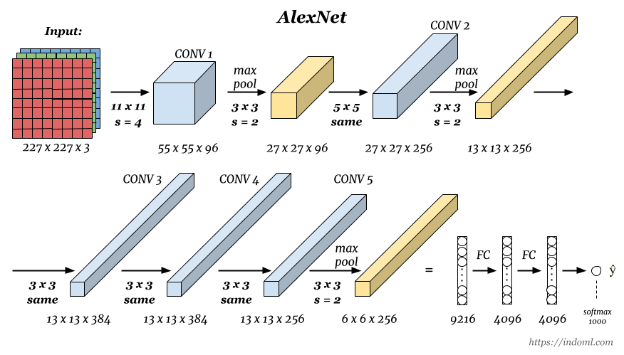
AlexNet was the winner of the ImageNet Large Scale Visual Recognition Challenge (ILSVRC) classification the benchmark in 2012.
Achieved 62.5% accuracy:

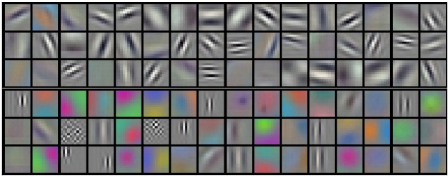
96 learnt filters:
9.2 VGG
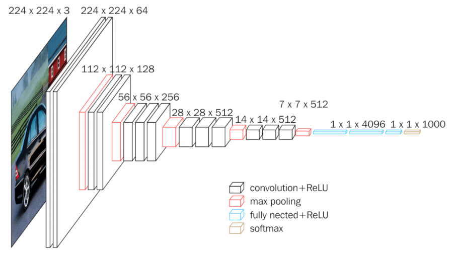
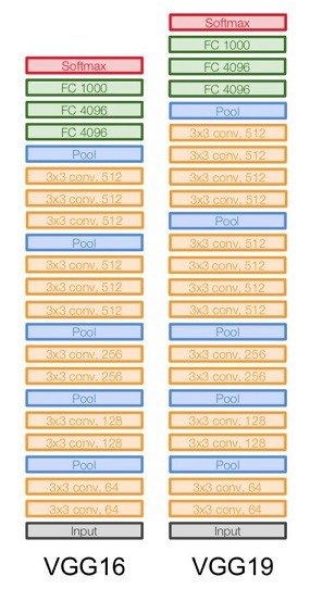
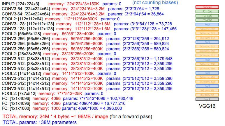
VGG-16 and VGG-19 (2014). The numbers 16 and 19 refer to the number of trainable layers. VGG-16 has \(\sim 138\) million parameters. VGGNet was the runner up of the ImageNet Large Scale Visual Recognition Challenge (ILSVRC) classification the benchmark in 2014.
9.3 ResNet
ResNet secured 1st Position in ILSVRC and COCO 2015 competition with an error rate of 3.6% (Better than Human Performance !!!) Batch Normalization after every conv layer. It also uses Xavier initialization with SGD + Momentum. The learning rate is 0.1 and is divided by 10 as validation error becomes constant. Moreover, batch-size is 256 and weight decay is 1e-5. The important part is there is no dropout is used in ResNet.
9.4 Inception
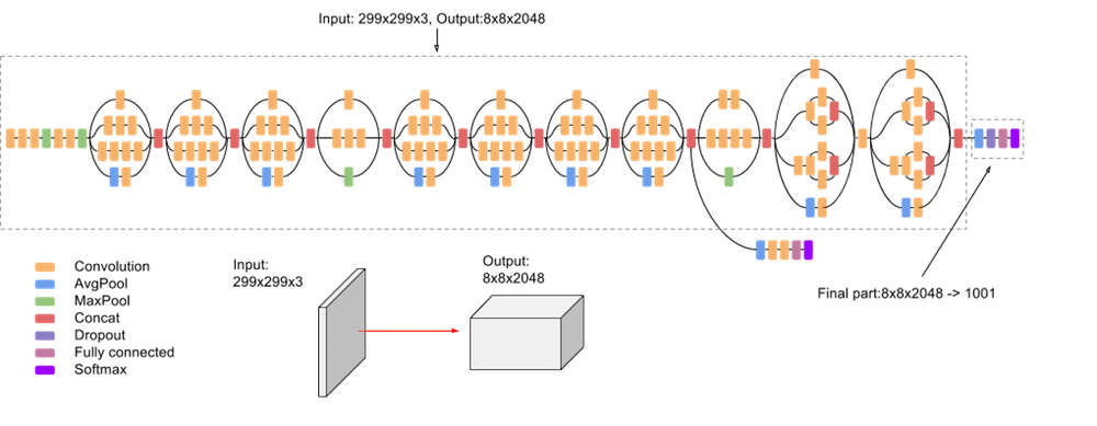
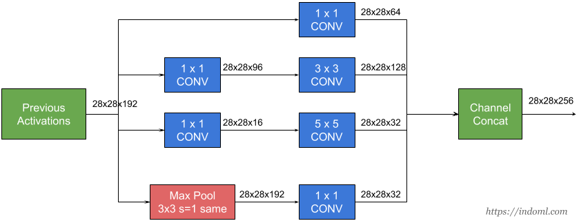
Inception-v3 with 144 crops and 4 models ensembled, the top-5 error rate of 3.58% is obtained, and finally obtained 1st Runner Up (image classification) in ILSVRC 2015. The motivation of the inception network is, rather than requiring us to pick the filter size manually, let the network decide what is best to put in a layer. GoogLeNet has 9 inception modules.
10 Document classification: IMDB movie reviews.
- The
IMDBcorpus consists of user-supplied movie ratings for a large collection of movies. Each has been labeled for sentiment as positive or negative. Here is the beginning of a negative review:
This has to be one of the worst films of the 1990s. When my friends & I were watching this film (being the target audience it was aimed at) we just sat & watched the first half an hour with our jaws touching the floor at how bad it really was. The rest of the time, everyone else in the theater just started talking to each other, leaving or generally crying into their popcorn…
We have labeled training and test sets, each consisting of 25,000 reviews, and each balanced with regard to sentiment.
We wish to build a classifier to predict the sentiment of a review.
10.1 Feature extraction: bag of words
Documents have different lengths, and consist of sequences of words. How do we create features \(X\) to characterize a document?
From a dictionary, identify the 10K most frequently occurring words.
Create a binary vector of length \(p = 10K\) for each document, and score a 1 in every position that the corresponding word occurred.
With \(n\) documents, we now have an \(n \times p\) sparse feature matrix \(X\).
We compare a lasso logistic regression model to a two-hidden-layer neural network on the next slide. (No convolutions here!)
Bag-of-words are unigrams. We can instead use bigrams (occurrences of adjacent word pairs), and in general \(m\)-grams.
10.2 Lasso versus neural network: IMDB reviews
11 Recurrent neural network (RNN)
Often data arise as sequences:
Documents are sequences of words, and their relative positions have meaning.
Time-series such as weather data or financial indices.
Recorded speech or music.
Handwriting, such as doctor’s notes.
RNNs build models that take into account this sequential nature of the data, and build a memory of the past.
The feature for each observation is a sequence of vectors \(X = \{X_1, X_2, \ldots, X_L\}\).
The target \(Y\) is often of the usual kind. For example, a single variable such as Sentiment, or a one-hot vector for multiclass.
However, \(Y\) can also be a sequence, such as the same document in a different language.
Schematic of a simple recurrent neural network.
In detail, suppose \(X_\ell^T = (X_{\ell 1}, X_{\ell 2}, \ldots, X_{\ell p})\) has \(p\) components, and \(A_\ell^T = (A_{\ell 1}, A_{\ell 2}, \ldots, A_{\ell K})\) has \(K\) components. Then the computation at the \(k\)th components of hidden unit \(A_\ell\) is \[\begin{eqnarray*} A_{\ell k} &=& g(w_{k0} + \sum_{j=1}^p w_{kj} X_{\ell j} + \sum_{s=1}^K u_{ks} A_{\ell-1,s}) \\ O_\ell &=& \beta_0 + \sum_{k=1}^K \beta_k A_{\ell k}. \end{eqnarray*}\]
Often we are concerned only with the prediction \(O_L\) at the last unit. For squared error loss, and \(n\) sequence/response pairs, we would minimize \[ \sum_{i=1}^n (y_i - o_{iL})^2 = \sum_{i=1}^n (y_i - (\beta_0 + \sum_{k=1}^K \beta_kg(w_{k0} + \sum_{j=1}^p w_{ij} x_{iLj} + \sum_{s=1}^K u_{ks}A_{i,L-1,s})))^2. \]
RNN and IMDB reviews.
The document feature is a sequence of words \(\{\mathcal{W}_\ell\}_1^L\). We typically truncate/pad the documents to the same number \(L\) of words (we use \(L = 500\)).
Each word \(\mathcal{W}_\ell\) is represented as a one-hot encoded binary vector \(X_\ell\) (dummy variable) of length 10K, with all zeros and a single one in the position for that word in the dictionary.
This results in an extremely sparse feature representation, and would not work well.
Instead we use a lower-dimensional pretrained word embedding matrix \(E\) (\(m \times 10K\)).
This reduces the binary feature vector of length 10K to a real feature vector of dimension \(m \ll 10K\) (e.g. \(m\) in the low hundreds.)
word2vec and GloVe are popular.After a lot of work, the results are a disappointing 76% accuracy.
We then fit a more exotic RNN, an LSTM with long and short term memory. Here \(A_\ell\) receives input from \(A_{\ell-1}\) (short term memory) as well as from a version that reaches further back in time (long term memory). Now we get 87% accuracy, slightly less than the 88% achieved by glmnet.
Leaderboard for IMDb sentiment analysis: https://paperswithcode.com/sota/sentiment-analysis-on-imdb.
12 LSTM
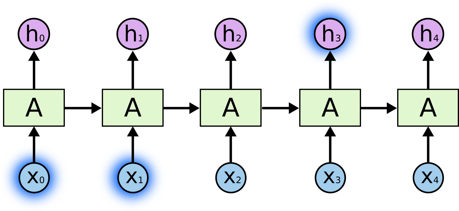
- Short-term dependencies: to predict the last word in “the clouds are in the sky”:
- Long-term dependencies: to predict the last word in “I grew up in France… I speek fluent French”:
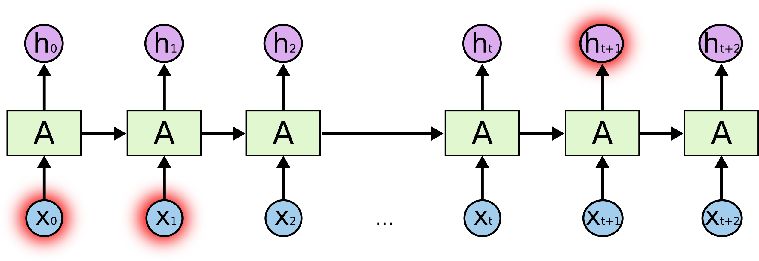
- Typical RNNs are having trouble with learning long-term dependencies.
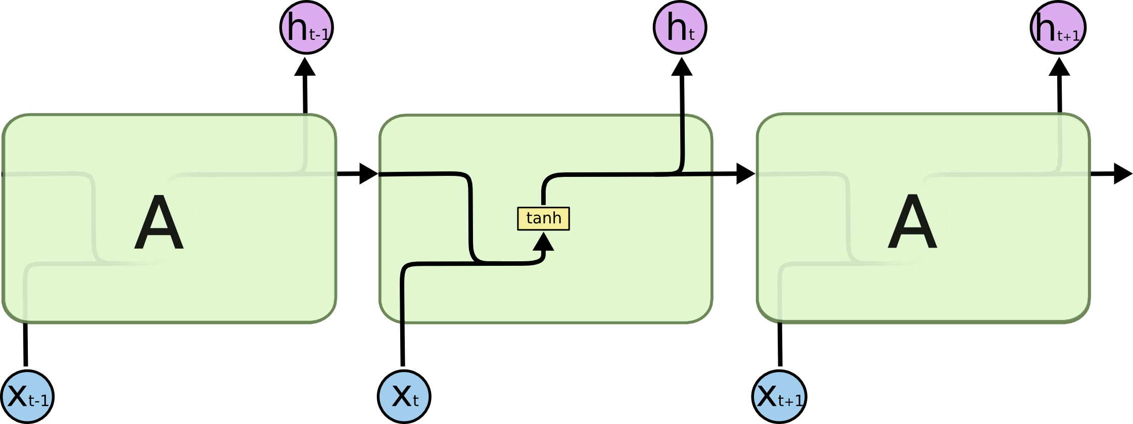
- Long Short-Term Memory networks (LSTM) are a special kind of RNN capable of learning long-term dependencies.
The cell state allows information to flow along it unchanged.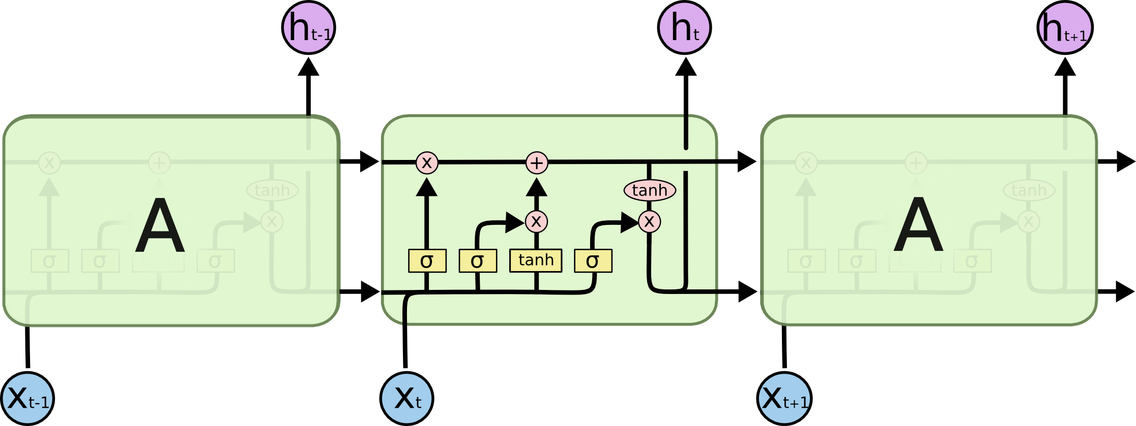

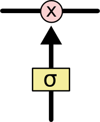
The gates give the ability to remove or add information to the cell state.
12.1 Transformers
13 NYSE (New York Stock Exchange) data
Three daily time series for the period Dec 3, 1962-Dec 31, 1986 (6,051 trading days).
Log trading volume: This is the fraction of all outstanding shares that are traded on that day, relative to a 100-day moving average of past turnover, on the log scale.Dow Jones return: This is the difference between the log of the Dow Jones Industrial Index on consecutive trading days.Log volatility: This is based on the absolute values of daily price movements.
The autocorrelation at lag \(\ell\) is the correlation of all pairs \((v_t, v_{t-\ell})\) that are \(\ell\) trading days apart.
These sizable correlations give us confidence that past values will be helpful in predicting the future.
13.1 RNN forecaster
We extract many short mini-series of input sequences \(X=\{X_1,X_2,\ldots,X_L\}\) with a predefied length \(L\) known as the
lag: \[\begin{eqnarray*} X_1 &=& \begin{pmatrix} v_{t-L} \\ r_{t-L} \\ z_{t-L} \end{pmatrix}, \\ X_2 &=& \begin{pmatrix} v_{t-L+1} \\ r_{t-L+1} \\ z_{t-L+1} \end{pmatrix}, \\ &\vdots& \\ X_L &=& \begin{pmatrix} v_{t-1} \\ r_{t-1} \\ z_{t-1} \end{pmatrix}, \end{eqnarray*}\] and \[ Y = v_t. \]Since \(T=6,051\), with \(L=5\) we can create \(6,046\) such \((X,Y)\) pairs.
We use the first 4,281 as training data, and the following 1,770 as test data. We fit an RNN with 12 hidden units per lag step (i.e. per \(A_\ell\).)
- \(R^2=0.42\) for RNN, \(R^2=0.18\) for straw man (use yesterday’s value of
log trading volumeto predict that of today).
13.2 Autoregression forecaster
The RNN forecaster is similar in structure to a traditional autoregression procedure. \[ y = \begin{pmatrix} v_{L+1} \\ v_{L+2} \\ v_{L+3} \\ \vdots \\ v_T \end{pmatrix}, M = \begin{pmatrix} 1 & v_L & v_{L-1} & \cdots & v_1 \\ 1 & v_{L+1} & v_{L} & \cdots & v_2 \\ \vdots & \vdots & \vdots & \ddots & \vdots \\ 1 & v_{T-1} & v_{T-2} & \cdots & v_{T-L} \end{pmatrix}. \]
Fit an OLS regression of \(y\) on \(M\), giving \[ \hat v_t = \hat \beta_0 + \hat \beta_1 v_{t-1} + \hat \beta_2 v_{t-2} + \cdots + \hat \beta_L v_{t-L}, \] known as an order-\(L\) autoregression model or AR(\(L\)).
For the NYSE data we can include lagged versions of
DJ_returnandlog_volatilityin matrix \(M\), resulting in \(3L+1\) columns.- \(R^2=0.41\) for AR(5) model (16 parameters)
- \(R^2=0.42\) for RNN model (205 parameter)
- \(R^2=0.42\) for AR(5) model fit by neural network
- \(R^2=0.46\) for all models if we include
day_of_weekof the day being predicted.
13.3 Summary of RNNs
We have presented the simplest of RNNs. Many more complex variations exist.
One variation treats the sequence as a one-dimensional image, and uses CNNs for fitting. For example, a sequence of words using an embedding representation can be viewed as an image, and the CNN convolves by sliding a convolutional filter along the sequence.
Can have additional hidden layers, where each hidden layer is a sequence, and treats the previous hidden layer as an input sequence.
Can have output also be a sequence, and input and output share the hidden units. So called
seq2seqlearning are used for language translation.
14 When to use deep learning
CNNs have had enormous successes in image classification and modeling, and are starting to be used in medical diagnosis. Examples include digital mammography, ophthalmology, MRI scans, and digital X-rays.
RNNs have had big wins in speech modeling, language translation, and forecasting.
Often the big successes occur when the signal to noise ratio is high, e.g., image recognition and language translation. Datasets are large, and overfitting is not a big problem.
For noisier data, simpler models can often work better.
On the
NYSEdata, the AR(5) model is much simpler than a RNN, and performed as well.On the
IMDBreview data, the linear model fit by glmnet did as well as the neural network, and better than the RNN.
We endorse the Occam’s razor principal. We prefer simpler models if they work as well. More interpretable!
15 Fitting neural networks

\[ \min_{w_1,\ldots,w_K,\beta} \quad \frac 12 \sum_{i=1}^n (y_i - f(x_i))^2, \] where \[ f(x_i) = \beta_0 + \sum_{k=1}^K \beta_k g(w_{k0} + \sum_{j=1}^p w_{kj} x_{ij}). \]
This problem is difficult because the objective is non-convex.
Despite this, effective algorithms have evolved that can optimize complex neural network problems efficiently.
15.1 Gradient descent
Let \[ R(\theta) = \frac 12 \sum_{i=1}^n (y_i - f_\theta(x_i))^2 \] with \(\theta = (w_1,\ldots,w_K,\beta)\).
Start with a guess \(\theta_0\) for all the parameters in \(\theta\), and set \(t = 0\).
Iterate until the objective \(R(\theta)\) fails to decrease:
(a). Find a vector \(\delta\) that reflects a small change in \(\theta\) such that \(\theta^{t+1} = \theta^t + \delta\) reduces the objective; i.e. \(R(\theta^{t+1}) < R(\theta^t)\).
(b). Set \(t \gets t+1\).
In this simple example we reached the global minimum.
If we had started a little to the left of \(\theta^0\) we would have gone in the other direction, and ended up in a local minimum.
Although \(\theta\) is multi-dimensional, we have depicted the process as one-dimensional. It is much harder to identify whether one is in a local minimum in high dimensions.
How to find a direction \(\delta\) that points downhill? We compute the gradient vector \[ \nabla R(\theta^t) = \frac{\partial R(\theta)}{\partial \theta} \mid_{\theta = \theta^t} \] and set \[ \theta^{t+1} \gets \theta^t - \rho \nabla R(\theta^t), \] where \(\rho\) is the learning rate (typically small, e.g., \(\rho=0.001\)).
Since \(R(\theta) = \sum_{i=1}^n R_i(\theta)\) is a sum, so gradient is sum of gradients. \[ R_i(\theta) = \frac 12 (y_i - f_\theta(x_i))^2 = \frac 12 (y_i - \beta_0 - \sum_{k=1}^K \beta_k g(w_{k0} + \sum_{j=1}^p w_{kj} x_{ij}))^2. \] For ease of notation, let \[ z_{ik} = w_{k0} + \sum_{j=1}^p w_{kj} x_{ij}. \]
Backpropagation uses the chain rule for differentiation: \[\begin{eqnarray*} \frac{\partial R_i(\theta)}{\partial \beta_k} &=& \frac{\partial R_i(\theta)}{\partial f_\theta(x_i)} \cdot \frac{\partial f_\theta(x_i)}{\partial \beta_k} \\ &=& - (y_i - f_\theta(x_i)) \cdot g(z_{ik}) \\ \frac{\partial R_i(\theta)}{\partial w_{kj}} &=& \frac{\partial R_i(\theta)}{\partial f_\theta(x_i)} \cdot \frac{\partial f_\theta(x_i)}{\partial g(z_{ik})} \cdot \frac{\partial g(z_{ik})}{\partial z_{ik}} \cdot \frac{\partial z_{ik}}{\partial w_{kj}} \\ &=& - (y_i - f_\theta(x_i)) \cdot \beta_k \cdot g'(z_{ik}) \cdot x_{ij}. \end{eqnarray*}\]
Two-pass updates: \[\begin{eqnarray*} & & \text{initialization} \to z_{ik} \to g(z_{ik}) \to \widehat{f}_{\theta}(x_i) \quad \quad \quad \text{(forward pass)} \\ &\to& y_i - f_\theta(x_i) \to \frac{\partial R_i(\theta)}{\partial \beta_k}, \frac{\partial R_i(\theta)}{\partial w_{kj}} \to \widehat{\beta}_{k} \text{ and } \widehat{w}_{kj} \quad \quad \text{(backward pass)}. \end{eqnarray*}\]
Advantages: each hidden unit passes and receives information only to and from units that share a connection; can be implemented efficiently on a parallel architecture computer.
Tricks of the trade
Slow learning. Gradient descent is slow, and a small learning rate \(\rho\) slows it even further. With early stopping, this is a form of regularization.
Stochastic gradient descent. Rather than compute the gradient using all the data, use a small minibatch drawn at random at each step. E.g. for
MNISTdata, with n = 60K, we use minibatches of 128 observations.An epoch is a count of iterations and amounts to the number of minibatch updates such that \(n\) samples in total have been processed; i.e. \(60,000/128 \approx 469\) minibatches for
MNIST.Regularization. Ridge and lasso regularization can be used to shrink the weights at each layer. Two other popular forms of regularization are dropout and augmentation.
15.2 Droptout learning
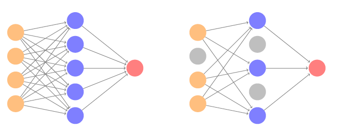
At each SGD update, randomly remove units with probability \(\phi\), and scale up the weights of those retained by \(1/(1-\phi)\) to compensate.
In simple scenarios like linear regression, a version of this process can be shown to be equivalent to ridge regularization.
As in ridge, the other units stand in for those temporarily removed, and their weights are drawn closer together.
Similar to randomly omitting variables when growing trees in random forests.
15.3 Ridge and data augmentation
Make many copies of each \((x_i, y_i)\) and add a small amount of Gaussian noise to the \(x_i\), a little cloud around each observation, but leave the copies of \(y_i\) alone!
This makes the fit robust to small perturbations in \(x_i\), and is equivalent to ridge regularization in an OLS setting.
Data augmentation is especially effective with SGD, here demonstrated for a CNN and image classification.
Natural transformations are made of each training image when it is sampled by SGD, thus ultimately making a cloud of images around each original training image.
The label is left unchanged, in each case still
tiger.Improves performance of CNN and is similar to ridge.

16 Double descent
With neural networks, it seems better to have too many hidden units than too few.
Likewise more hidden layers better than few.
Running stochastic gradient descent till zero training error often gives good out-of-sample error.
Increasing the number of units or layers and again training till zero error sometimes gives even better out-of-sample error.
What happened to overfitting and the usual bias-variance trade-off?
Belkin, Hsu, Ma and Mandal (2018) Reconciling Modern Machine Learning and the Bias-Variance Trade-off. arXiv
16.1 Simulation study
Model: \[ y= \sin(x) + \epsilon \] with \(x \sim\) Uniform(-5, 5) and \(\epsilon\) is Gaussian with sd=0.3.
Training set \(n=20\), test set very large (10K).
We fit a natural spline to the data with \(d\) degrees of freedom, i.e., a linear regression onto \(d\) basis functions \[ \hat y_i = \hat \beta_1 N_1(x_i) + \hat \beta_2 N_2(x_i) + \cdots + \hat \beta_d N_d(x_i). \]
When \(d = 20\) we fit the training data exactly, and get all residuals equal to zero.
When \(d > 20\), we still fit the data exactly, but the solution is not unique. Among the zero-residual solutions, we pick the one with minimum norm, i.e. the zero-residual solution with smallest \(\sum_{j=1}^d \hat \beta_j^2\).
When \(d \le 20\), model is OLS, and we see usual bias-variance trade-off.
When \(d > 20\), we revert to minimum-norm solution. As \(d\) increases above 20, \(\sum_{j=1}^d \hat \beta_j^2\) decreases since it is easier to achieve zero error, and hence less wiggly solutions.
Some facts.
In a wide linear model (\(p \gg n\)) fit by least squares, SGD with a small step size leads to a minimum norm zero-residual solution.
Stochastic gradient flow, i.e. the entire path of SGD solutions, is somewhat similar to ridge path.
By analogy, deep and wide neural networks fit by SGD down to zero training error often give good solutions that generalize well.
In particular cases with high signal-to-noise ratio, e.g., image recognition, are less prone to overfitting; the zero-error solution is mostly signal!
17 Generative Adversarial Networks (GANs)
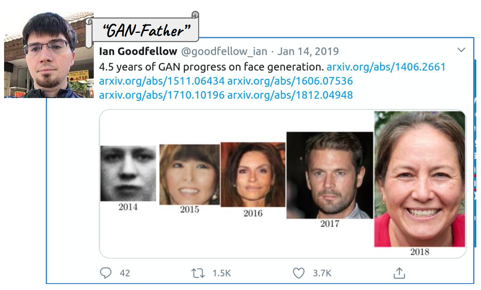
The coolest idea in deep learning in the last 20 years.
- Yann LeCun on GANs.
Sources:
Applications:
AI-generated celebrity photos: https://www.youtube.com/watch?v=G06dEcZ-QTg
Digital art: Edmond de Belamy
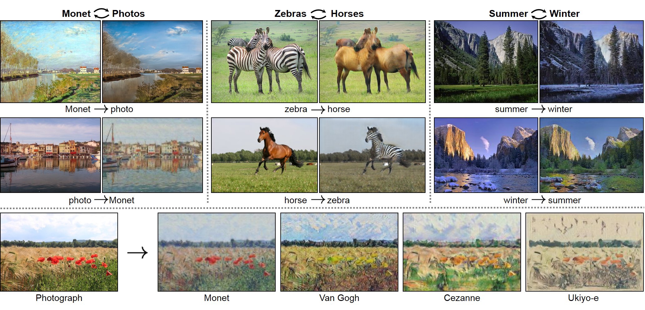
Image-to-image translation
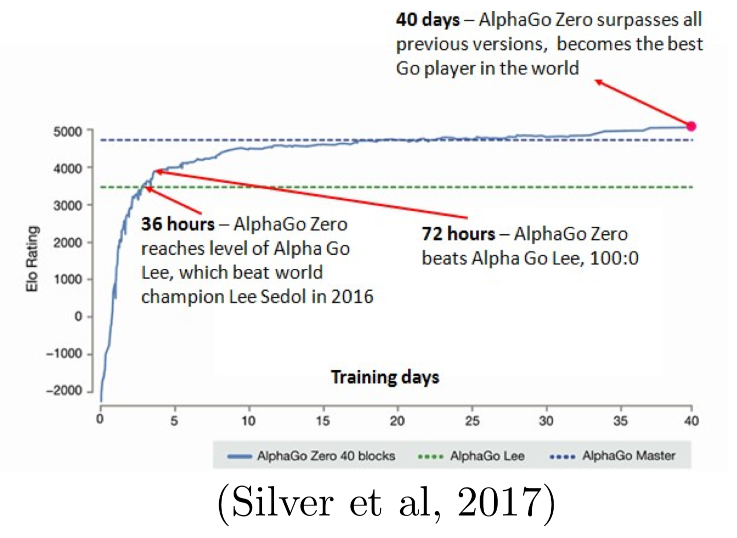
- Self play
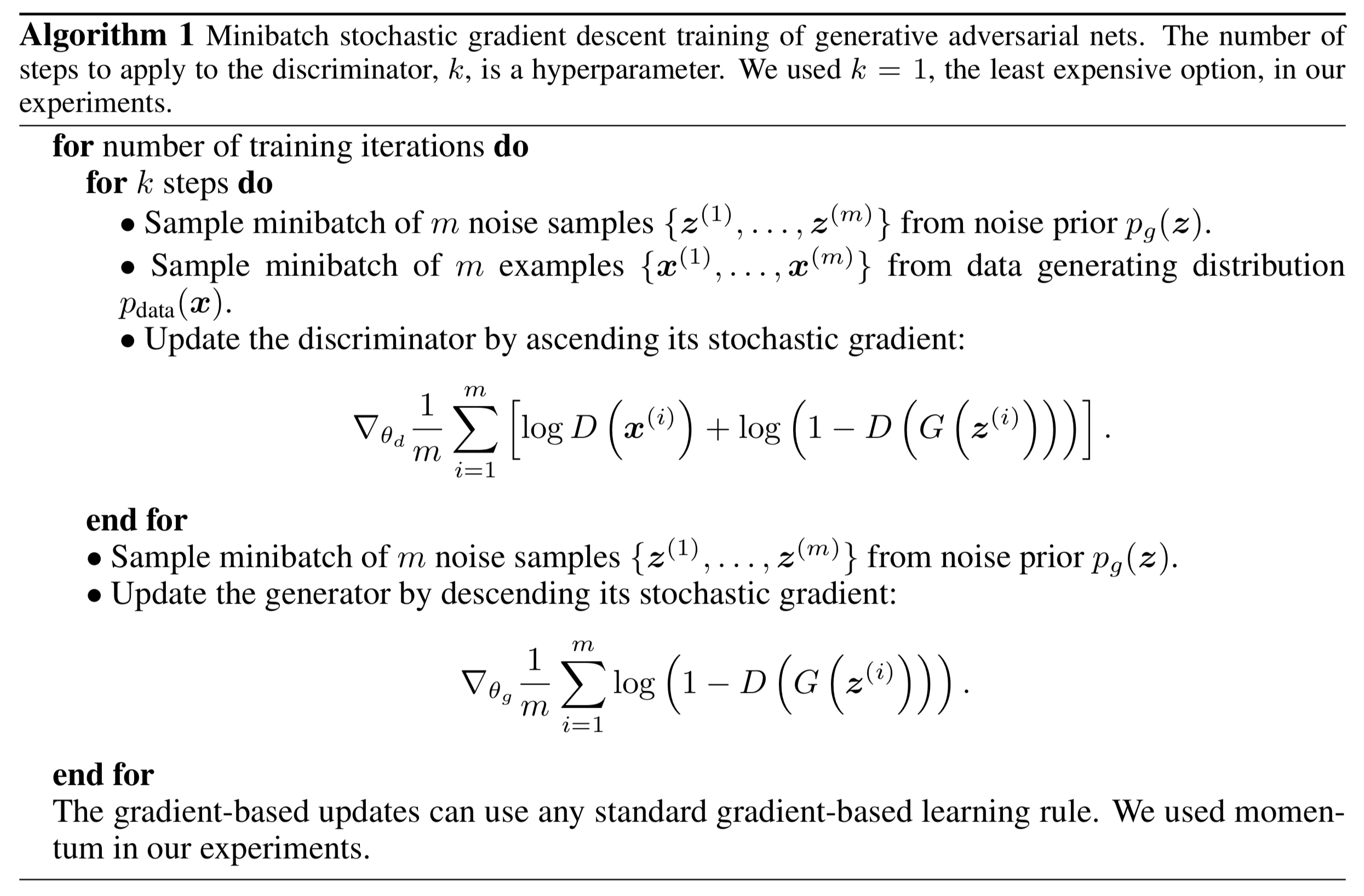
- GAN:
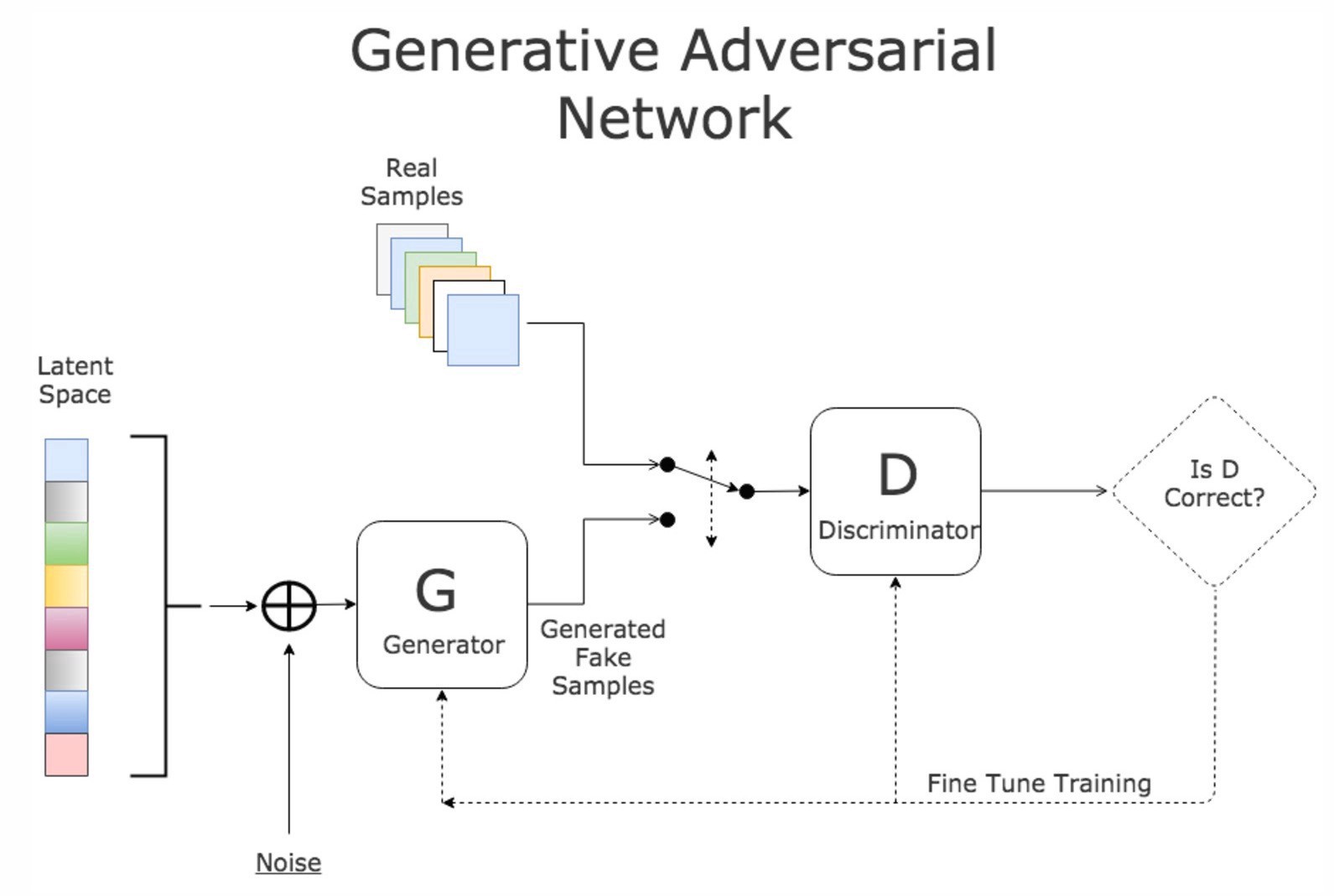
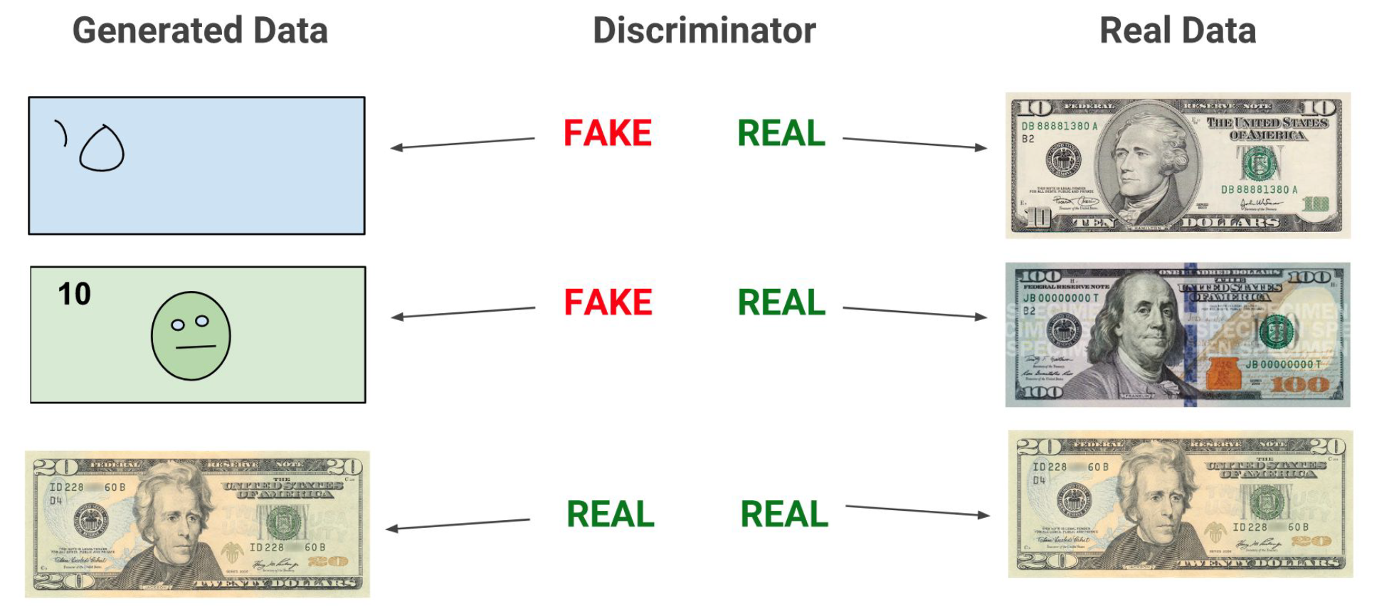
Value function of GAN \[ \min_G \max_D V(D, G) = \mathbb{E}_{x \sim p_{\text{data}}(x)} [\log D(x)] + \mathbb{E}_{z \sim p_z(z)} [\log (1 - D(G(z)))]. \]
Training GAN
